We continue our series on generative AI. We have discussed Transformers, large language models, and some specific aspects of Transformers – but are modern LLMs still running on the exact same Transformer decoders as the original GPT? Yes and no; while the basics remain the same, there has been a lot of progress in recent years. Today, we briefly review some of the most important ideas in fine-tuning LLMs: RLHF, LoRA, instruction tuning, and recursive self-improvement. These ideas are key in turning a token prediction machine into a useful tool for practical applications.

From GPT to GPT-4: What Has Been Changing?

For over a year, I have been writing about generative AI on this blog. Recently, we have discussed the basic architecture of this latest generative AI revolution: the Transformer. We have also considered modern LLMs and even reasons to worry about their future development, and we have discussed in detail one specific venue of progress: how to extend the context window size in Transformers, alleviating the quadratic complexity of self-attention.

But has this fight for context windows been the entire difference between the original Transformer and the latest GPT-4, Gemini 1.5, and the rest? Is there anything else except for “stacking more layers”? Sure there is, and today we discuss it in more detail.

Before proceeding further, I have to warn you that the new ideas and especially engineering implementation details of the very latest large language models are not being released to the public. There is no definitive paper about GPT-4’s internal structure (let alone plans for GPT-5) written by OpenAI researchers. Still, there are plenty of ideas floating around, and plenty of information already available from previous attempts by leading labs, from publicly released models such as the Llama family, and from independent research efforts. 

So while I’m not claiming to show you the full picture today, I still hope to give a wide enough survey. Our plan is as follows:

• we begin with the most important advance that made GPT-3 into ChatGPT and kickstarted the LLM revolution: reinforcement learning with human feedback (RLHF);
• then we discuss fine-tuning pretrained LLMs on small datasets by learning adapters for the mostly frozen weights of the base models; the most popular and efficient tool here have been low-rank adapters (LoRA);
• next, we consider instruction tuning, where LLMs are themselves fine-tuned on datasets providing realistic prompt-response samples rather than token prediction in arbitrary text; the main question here is where to get the data, and we discuss both manually labeled datasets and our main focus, synthetic data;
• finally, synthetic data for LLM fine-tuning and reinforcement learning come together in our last topic: attempts at recursive self-improvement where the LLM may become smarter by bootstrapping from its own outputs.

All of these techniques, and more, are key to efficiently using LLMs for practical problems, especially for specific applications such as mathematical reasoning or programming; we will see many such examples below.

Giving Humans What They Want: RLHF

You have certainly heard of reinforcement learning with human feedback (RLHF). This is the secret sauce that turned GPT-3, an amazing but hard to use token prediction machine, into ChatGPT, an LLM that keeps turning the world upside down. But how does it work, exactly?

We don’t often talk about reinforcement learning (RL) on this blog; probably the only notable exception was my last post on world models, where RL was featured very prominently. In general, it is a separate way of doing machine learning, in addition to supervised and unsupervised learning:

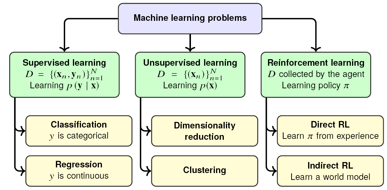
In supervised learning, you have a labeled dataset and want to learn a conditional distribution of labels given the data points. In unsupervised learning, there are no labels, you just mine the data for structure, learning the joint distribution of all variables. For example, token prediction is pure classification, a supervised learning problem of learning p(y|x) for a text prompt x and next token y, but we can also say that as a result, the language model has implicitly learned a distribution over text snippets p(x) because it can generate whole texts in an autoregressive fashion. 

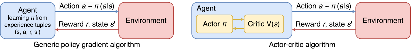
In reinforcement learning, there is no prior dataset: a learning agent is just “living” in an environment, getting rewards based on actions that it takes and trying to maximize these rewards. In the last post, we discussed the distinction between several different approaches to RL such as policy gradient and actor-critic algorithms:

But be it with a world model or without, RL and training an LLM sound very different, right?

RLHF started with the work of OpenAI researchers Christiano et al. (2017). Paul Christiano is one of the leading figures in the field of AI alignment, and this work was also motivated by a problem that sounds more like alignment: how do we tell, for instance, a robot what exactly we want it to do? Unless we are in a self-contained formal system such as chess, any reward function that we could formulate in the real world might be superficially optimized in ways that are hard to predict but that do not give us what we want. It is well known, for example, that robots learning complex behaviors in simulated environments often learn more about the bugs and computational limits of the simulator than about the desired behavior in the real world; for more details see, e.g., Lehman et al., 2018 or a list of specification gaming examples by Krakovna et al..

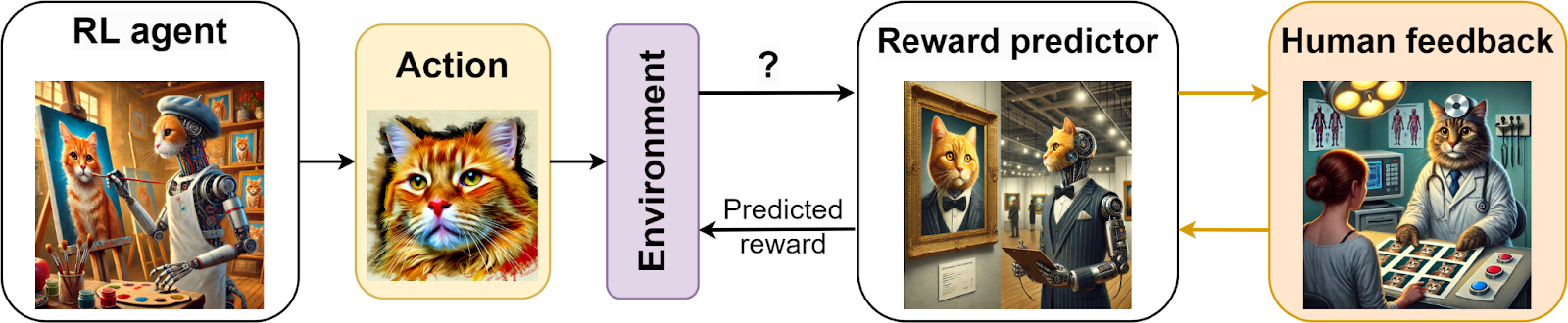
Thus, Christiano et al. suggested that since we most probably cannot define what we want formally, we can instead ask a human: when you see it, you know it. Human feedback would define how well the system’s current behavior matches the actual hard-to-define goal; that feedback might be provided in the form of comparing two responses or two outcomes and preferring one of them. This approach, however, is impractical: we cannot ask humans to label as much data as actually necessary to train a reinforcement learning model. Therefore, the idea of Christiano et al. is to train a separate model that encodes user preferences and predicts the reward used in actual RL training. Here is a general scheme of this training:

The human providing feedback cannot assign numerical reward value, so instead they compare pairs of “actions”—in the case of Christiano et al., actions were short sequences of Atari game playing or a robot walking—and give pairwise preferences. As a result, the dataset looks like a set of pairs D={(σ₁, σ₂, μ)_n}_n=1^N, where σ_i = ((o_i0, a_i0), (o_i1, a_i1), …, (o_{i,k_i}, a_{i,k_i})) are sequences of observation-action pairs that describe a trajectory in the reinforcement learning environment, and μ is a probability distribution specifying whether the user preferred σ₁, σ₂, or had an equal preference (uniform μ). 

To convert pairwise preferences into a reward function, this approach uses the assumptions of Bradley–Terry models for learning a rating function from pairwise preferences (Bradley, Terry, 1952). The problem setting for a Bradley–Terry model is a set of pairwise comparisons such as the results of, e.g., chess games between players, and the basic assumption is that the probability of player i winning over player j can be modeled as

for some rating values ɣ_i,ɣ_j∊ℝ. Then Bradley–Terry models provide algorithms to maximize the total likelihood of a dataset with such pairwise comparisons, usually based on minorization-maximization algorithms, a generalization of the basic idea of the EM algorithm (Hunter, 2004; see also a discussion of EM below).

In the case of RL from human preferences, we need a further assumption since ɣ_i has to be a function of σ_i; Christiano et al. (2017) modeled it as a product of exponential rewards over the sequence:

and then the loss function for the neural network can be defined as

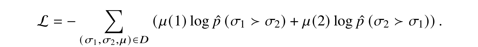
It might seem that this idea just shifts the impractical part of providing human feedback during RL training to an equally impractical task of providing enough human feedback to train a reward prediction model. However, it turned out that with this approach, it only takes a few hundred queries to a human rater to learn walking or hopping in the MuJoCo simulated environment (Todorov et al., 2012; see a sample choice posed for the human evaluator on the left in the figure below), and if you are willing to go over 1000 queries you might even get better results than pure reinforcement learning! The latter effect is probably due to reward shaping (Wiewiora, 2010): when we humans rate behaviors, we impose an ordering where sequences closer to the goal are rated higher, and the resulting rewards provide more information to the agent than just a binary label of whether the task has been done successfully.

By the way, this work also contains a very interesting example of reinforcement learning gone rogue. On the right, the figure above shows a sample frame from a video showing the robotic hand trying to grasp the ball. Human evaluators were asked to check whether the grasping had been successful. But since the scene had only one virtual camera, and with such a uniform background depth estimation was hard for humans, the robot learned to position the hand between the ball and the camera so as to appear as if it is grasping the ball rather than actually doing it! This is an excellent example of what is known as specification gaming, when machine learning models converge on behaviors that had not been intended by the developers but that indeed optimize the objective function they specified; we have talked about possible problems resulting from such effects on the blog before.

The ideas of Christiano et al. have been continued in many works. In particular, there have been extensions to k-wise comparisons, with a specially developed maximum likelihood estimator (Zhu et al., 2023), to vague feedback, where a human evaluator can only reliably distinguish two samples if their quality differs significantly (Cai et al., 2023), and to multi-agent systems (Ward et al., 2022). On the other hand, this direction of research can be placed in a theoretical framework of preference-based reinforcement learning (PbRL), where reward values are replaced with preferences (Fürnkranz et al., 2012; Jain et al., 2015; Wirth et al., 2017; Xu et al,. 2020).

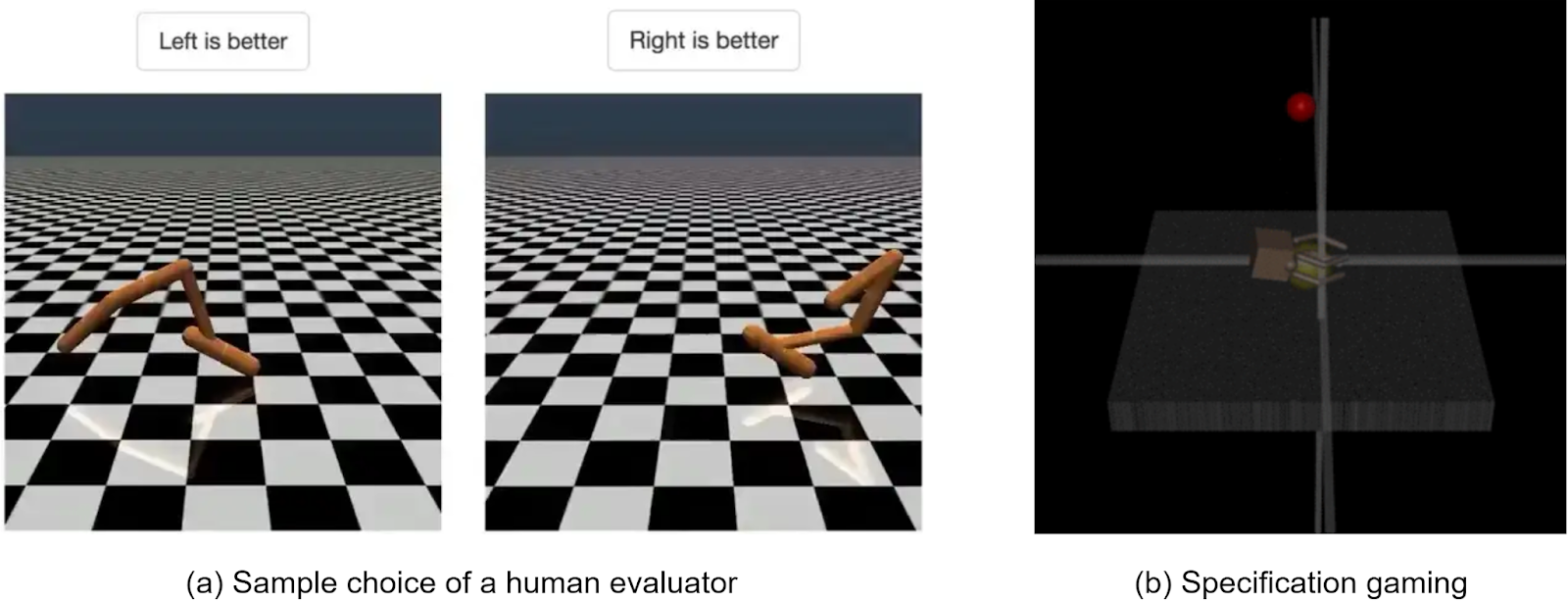
But the most important continuation was, of course, RLHF itself, an application of deep RL from human preferences to large language models. The first step was taken in 2020, when OpenAI researchers Stiennon et al. (2020) developed a summarization model based on human feedback. Their approach, illustrated in the figure below, is very similar: they collect human feedback on which document summaries are better, train a reward model to match these preferences, and then use the reward model to fine-tune with reinforcement learning.

For training the reward model, they change the loss function we have discussed above to a classification loss based on the logistic sigmoid:

where y₁ and y₂ are two summaries of the text x, and μ is 0 or 1 depending on which one the user prefers. For reinforcement learning, they used proximal policy optimization (PPO), a standard policy gradient RL algorithm that we will not describe here in detail; see, e.g., (Schulman et al., 2017; Sutton, Barto, 2018; Zheng et al., 2023). 

One important remark here is that if the reinforcement learning process is left unchecked, it is very likely to overfit, diverge very significantly from the original model, and collapse into a single node since human feedback is, of course, too scarce for full-scale training. Therefore, RLHF adds a penalty term in the reward function r(x,y) that urges the learned policy π_RL to not differ too significantly from the original supervised model π_SFT, usually in the form of KL divergence between the two:

The real revolution in LLMs came when OpenAI researchers Ouyang et al. (2022) applied this direction of research directly to large language models. Their goal was to make LLMs from the GPT-3 family (Brown et al., 2020) useful and user-friendly. The problem is that by default, a token prediction machine is merely giving you a plausible continuation for a text stream. It is not “trying” to be helpful, inoffensive, or even truthful because continuations such as lying, evading the question, or redirecting the conversation to a new topic also may be just as plausible from the point of view of the training set (which strives to include all meaningful text scraped off the Web) as truthfully and fully answering the user’s question.

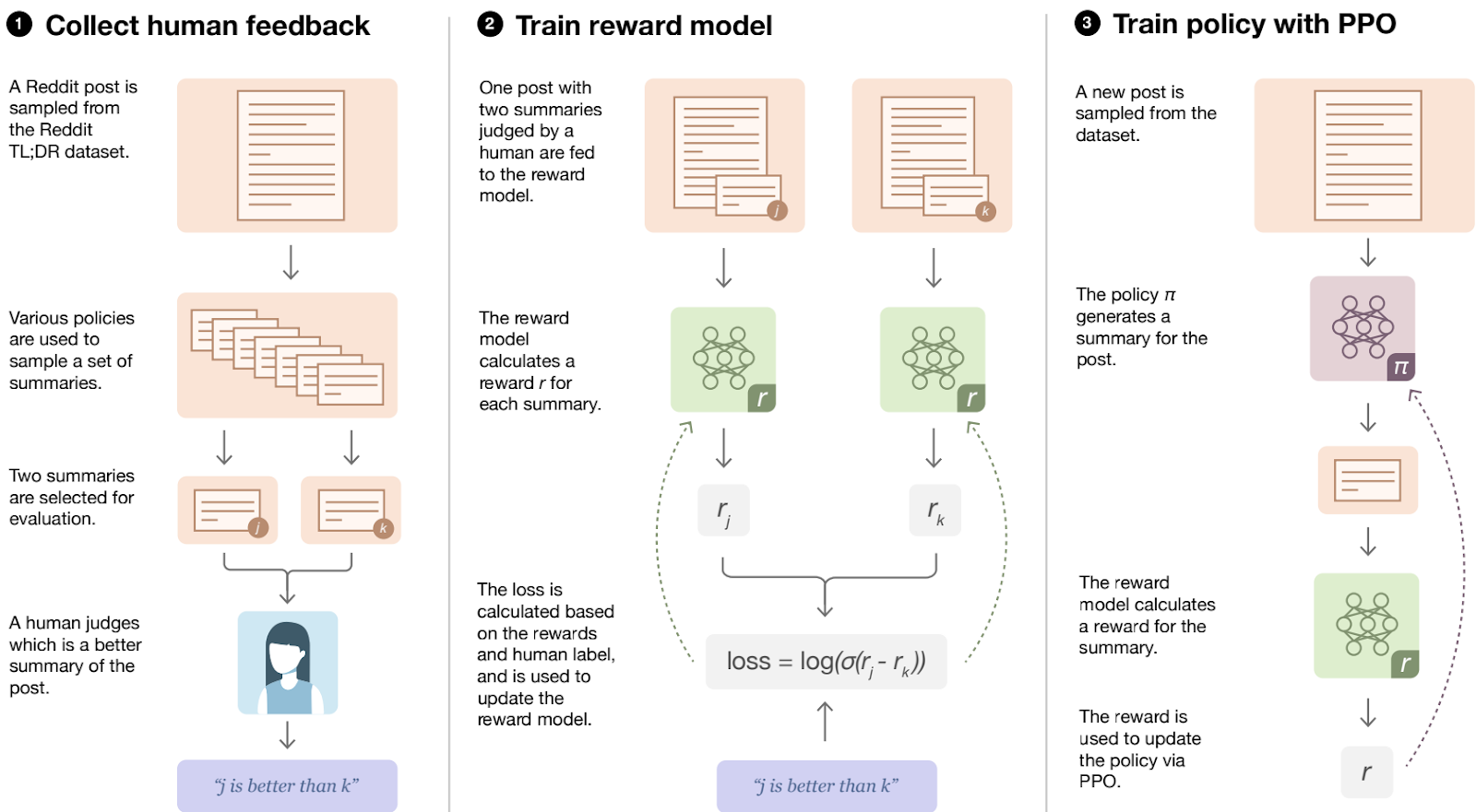
Therefore, Ouyang et al. (2022) applied RLHF, as described above, to the outputs of a large language model; the overall structure of this approach, illustrated in the figure below, is very similar to RLHF for summarization shown above:

This time, human evaluators are asked to decide which of the model’s outputs are most helpful, least offensive, and most truthful. The resulting LLM, InstructGPT, was reported to significantly gain in truthfulness, toxicity, and following instructions and explicit constraints in the prompt; the improvements were also quite robust and generalized even to languages not present in the human feedback dataset (Ouyang et al., 2022; OpenAI blog).

After InstructGPT, there was only a short step left to ChatGPT. InstructGPT was published in January 2022, and in November, OpenAI published a follow-up introducing a model that was also fine-tuned by RLHF but with an emphasis on conversation (OpenAI, 2022). For ChatGPT, human trainers held prolonged conversations with the model, and human feedback consisted in evaluating entire conversations rather than individual responses to requests; other than that, ChatGPT followed the exact same RLHF method. RLHF set off improvements in making LLMs useful, and the rest was history: the release of ChatGPT set off the “Spring of AI” in 2023 (see our previous post) and the wave of LLM research that we are still experiencing today. We have already discussed this wave, and will probably continue to do so in the future, but now we proceed to a different way to fine-tune LLMs.

Low-Resource Fine-Tuning via Approximations: LoRA

In a previous post on extending context windows for Transformers, we saw a number of methods that alleviate quadratic complexity based on low-rank approximations. A similar set of techniques can also be adapted for faster and less memory-intensive fine-tuning.

Low-rank adaptation (LoRA) is a technique designed to fine-tune large pretrained models efficiently by reducing the number of trainable parameters via low-rank approximations. Introduced by Microsoft researchers Hu et al. (2021), it begins with the classical idea of a low-rank decomposition for a matrix, as illustrated below: a large N⨉M matrix X is approximated with a product of two rectangular matrices,

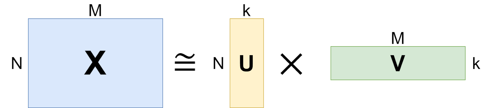
The product UV s, by construction, a matrix of rank k, and there exist efficient algorithms for finding U and V such that UV is the best approximation to X of rank k, where “best” is usually understood in terms of the L₂-norm of the difference, ‖X–UV‖₂.

In machine learning, methods based on low-rank approximations have a long history and are always very tempting: if you can assume that a large matrix you are interested in has rank k, you can replace the O(NM) complexity of learning it with the O((N+M)k) complexity of learning the matrices U and V, virtually free of charge. For large language models and large neural networks in general, there had been prior research that showed that the space of parameters in large models is usually too large:

• Li et al. (2018) introduced the notion of intrinsic dimension by training neural networks in random subspaces of the parameter space with gradually increasing dimension; they showed that the dimension when solutions begin to appear is inevitably much smaller than the number of parameters, often surprisingly so;
• Aghajanyan et al. (2021) applied this concept to fine-tuning language models, showing that standard pretrained models such as RoBERTa have very low intrinsic dimensions, which means that a little fine-tuning in the right subspace can go a very long way.

This last point is exactly what LoRA is about. LoRA makes the assumption that changes introduced by fine-tuning can be represented with a matrix of low rank. In other words, it fixes the pretrained matrix of weights W∈ℝ^N⨉M and looks for a ΔW in the form of a low-rank approximation ΔW = BA, where B∈ℝ^N⨉k, A∈ℝ^k⨉M.

For training, LoRA uses a random Gaussian initialization for A and zero for B, which means that at the start of training, ΔW is zero. Then you just fine-tune the model with your new dataset and use W+ΔW as the new weight matrix.

By focusing on low-rank updates, LoRA drastically reduces the computational and memory overhead compared to traditional fine-tuning methods. Hu et al. (2021) note that even very small values of k suffice; for example, they list a LoRA checkpoint for the large Transformer model with k=4 and only query and value weight matrices being modified, thus bringing the checkpoint size down from 350GB for the full weight matrix to 35MB, a 10000x reduction!

After training, there is technically no need to store A and B, you can just use the modified weight matrix W’=W+ΔW since you have to store the N⨉M weight matrix anyway. But with LoRA, you can have several different fine-tunings, for a variety of additional datasets and expected effects, applied to the same base weight matrix W. You only have to store the base matrix once and store new variations as a collection of different A_i and B_i, as illustrated below:

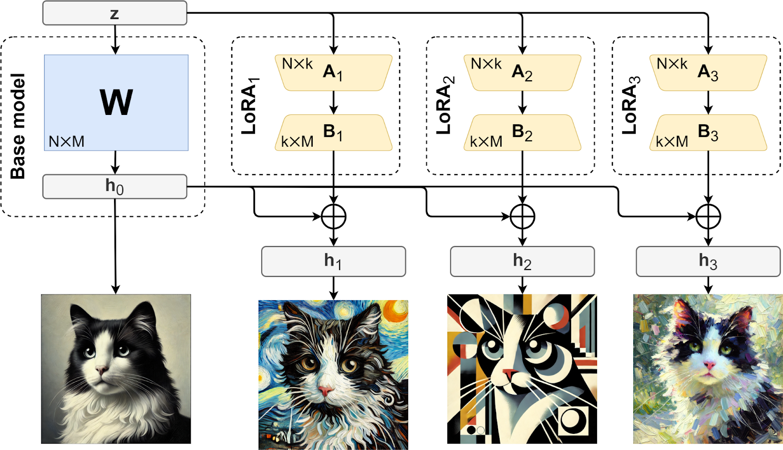
Low memory footprint and much reduced computational requirements for training also make it possible to train LoRA updates even to large models on consumer-grade hardware, without expensive clusters or even multiple GPUs. This has already led to the creation of cottage industries of various LoRA-based modifications for openly released image generation models, especially Stable Diffusion (Rombach et al., 2022), and large language models, especially the Llama family (Touvron et al., 2023a; 2023b).

LoRA was introduced in 2021, so naturally, there has already been a lot of research that expands upon these ideas. Let us survey a few important novel LoRA extensions.

First, an important problem in any low-rank approximation scheme is how to choose the rank k. If it is too high, we are wasting computation and memory, but if it is too low, we are losing valuable expressive power that would cost very little. 

Therefore, many extensions of LoRA concentrate on how to choose the rank k in some automated way:

• adaptive low-rank adaptation (AdaLoRA; Zhang et al., 2023) parametrizes ΔW as a proper singular value decomposition, ΔW = PΛQ, where matrices P∈ℝ^N⨉k and Q∈ℝ^k⨉M  are now orthogonal, and Λ = diag(λ₁, λ₂, …, λ_k) is a diagonal matrix of singular values; in SVD, the magnitudes of singular values |λ_i| are representative of the significance of the corresponding additional components in the decomposition, and one can prune singular values of low magnitudes; note, however, that running a full SVD on matrices of size N⨉M on every step would be too computationally intensive, so AdaLoRA approximates the decomposition by adding orthogonality regularizers on P and Q to the loss function:
  
• sparse low-rank adaptation (SoRA; Ding et al., 2023) notes that the relevant part of the SVD decomposition is that the matrix Λ serves as a gating mechanism for rows and columns of A and B: if a singular value is zero the corresponding dimension can be removed; therefore, they make this gating stage explicit, considering ΔW as the composition with a componentwise multiplication in the middle,
  
  and then optimize the components of g with a sparsity-inducing L₁ regularizer;
• allocating low-rank adaptation (ALoRA; Liu et al., 2024) also adds a diagonal matrix Λ in between A and B but does not try to make A and B orthogonal; instead, it proposes a separate ablation algorithm AB-LoRA to evaluate the importance of individual ranks in Λ, and then prunes ranks with low importance or increases the dimension of matrices where every rank is important; note that here, as usual in LoRA approaches, the ΔW = BA decomposition is done separately for different weight matrices in the network, and ranks may differ across them;
• dynamic search-free low-rank adaptation (DyLoRA; Valipour et al., 2023) samples the rank k on every training step and trains the truncated versions of A and B; the authors show that this approach can lead to significant time savings in LoRA training;
• weight-decomposed low-rank adaptation (DoRA; Liu et al., 2024) decomposes each pretrained weight into two components, magnitude and direction, and tunes them separately; formally this means that the weight matrix W gets decomposed as W = ‖W‖ · ( W / ‖W‖ ), and LoRa is applied only to the directional part:
  
  this can reduce the number of trainable parameters, and the authors show that it matches or surpasses basic LoRa in various tasks at no additional training cost.

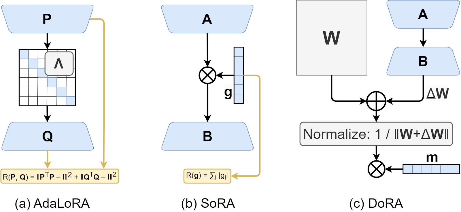
Here is an illustration of several LoRA variations:

Overall, low-rank adaptation is one of the most popular ways to fine-tune existing large models: even a very small dataset may be enough to train a low-rank adapter, and the resulting model can still use all of the power of the large number of pretrained weights. But it’s not the only way, so let us press on.

Instruction Tuning and Where to Get the Data for It

For large language models, both RLHF and low-rank adaptation usually aim to bridge the gap between pretext tasks, i.e., tasks that the LLM pretrains on, and actual use cases that involve fulfilling user requests in the form of natural language prompts. The archetypal pretext task is predicting the next token, but the tasks posed by humans may look very different.

Therefore, it often makes sense to fine-tune a large language model with a dataset specifically providing realistic examples of instructions and proper responses, a process known as instruction tuning. Here is a general illustration of the instruction tuning process from a recent survey by Zhang et al., (2024):

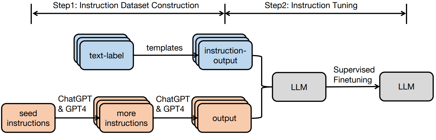
Actually, the tuning itself (Step 2 in the figure) is more or less trivial: you just fine-tune the model on a new dataset of inputs and outputs. The interesting part here is usually the dataset construction: where can you get a lot of input-output pairs with realistic instructions and responses? There are several different approaches:

First, you could always use human labeling: the required dataset size is not that large and manual labeling is often feasible. For example, we have discussed above how Ouyang et al. (2022) trained InstructGPT; we discussed it in the context of RLHF but recall that the first step there was exactly instruction tuning, i.e., supervised fine-tuning (SFT) on a dataset of natural language instructions. For InstructGPT, the SFT dataset contained about 13K training prompts, and the dataset used to train the reward model had about 33K more—not something you can label by yourself over an evening but still eminently feasible. OpenAI used a combination of handcrafted manual labeling and real prompts from their API.

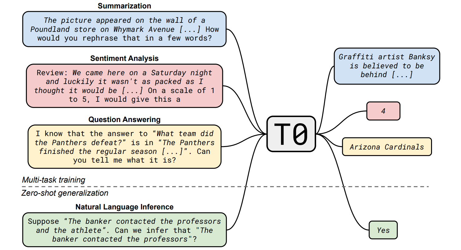
There already exist a number of public datasets for fine-tuning LLMs. Several of them were intended to make LLMs (and perhaps other models) to better generalize to unseen tasks. Sanh et al. (2022) put it as follows in their paper on one such dataset, P3 (Public Pool of Prompts): “An influential hypothesis is that large language models generalize to new tasks as a result of an implicit process of multitask learning… learning to predict the next word, a language model is forced to learn from a mixture of implicit tasks”. So these datasets make the multitask learning explicit rather than implicit, specifying a wide variety of tasks in the hope that the fine-tuned model will not only do well on those but also will generalize to new tasks when given similar zero-shot instructions. Here is an illustration with sample tasks by Sanh et al. (2022):

With this approach, one can adapt already existing NLP datasets for various tasks, providing one or a few descriptions for every task and thus turning a dataset previously designed to train NLP models from scratch into a prompt-response dataset suitable for fine-tuning LLMs. P3 combined at least a couple dozen different datasets, and later another couple dozen were added by Muenninghof et al. (2022) who published xP3, a multilingual version of P3 that not only contains more data but also can provide similar tasks in different languages. A similar dataset is Flan 2022 (Longpre et al., 2023), a collection of data for auxiliary tasks used to train the Flan-T5 model (Chung et al., 2022).

Another important example is Natural Instructions by Mishra et al. (2022), later extended to Super-Natural Instructions by Wang et al. (2022); they employed crowdsourcing labelers to generate questions about text snippets and also answer them in order to make LLMs (or other models) generalize better to unseen tasks, use common sense and common knowledge better, and so on. Here are some sample questions from these datasets:

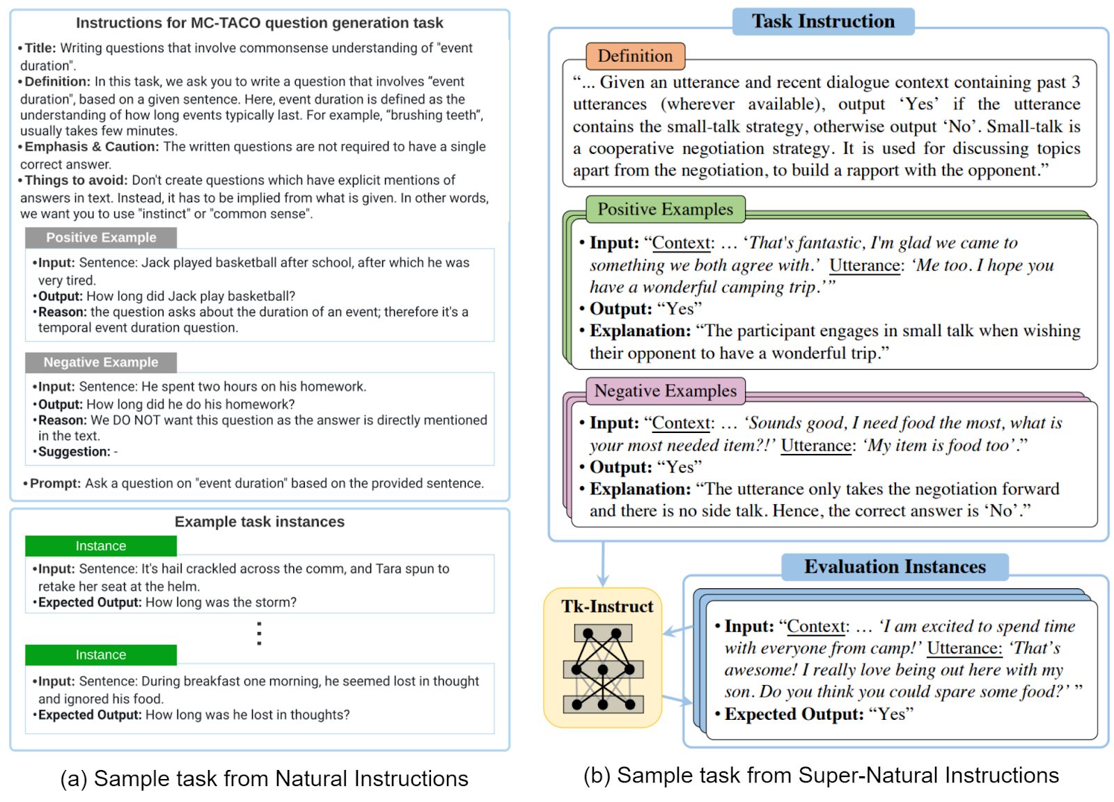
Natural Instructions, by the way, can also illustrate the limitations of crowdsourcing. I went to the dataset website and explored the commonsense event duration example, shown on the left in the figure above. Literally the first example I found there looked like this: 

• Input: Sentence: Islam later emerged as the majority religion during the centuries of Ottoman rule, though a significant Christian minority remained. 
• Output: What day did Islam emerge as the majority religion?

Not the most meaningful of questions, and I’m pretty sure it wasn’t intended by the original instructions…

A dataset even more directly related to LLMs and instruction tuning is databricks-dolly (Conover et al., 2023). It contains over 15000 records manually created by DataBricks employees for different categories of instruction following questions similar to those used in InstructGPT; unlike OpenAI’s datasets, this one is freely available for download, as well as the Dolly LLM fine-tuned on it. Another similar effort is LIMA (Less Is More for Alignment; Zhou et al., 2023), an interesting experiment where the authors fine-tune LLaMA-65B (as the name suggests, it has 65 billion parameters) with only 1000 curated prompt-response pairs, achieving very good results.

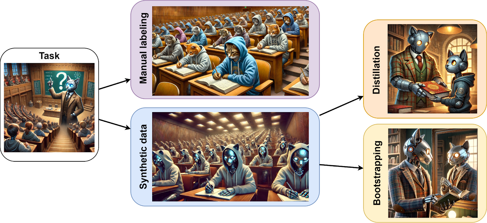
These are some of the manually labeled datasets. But, of course, here we have a great opportunity to circle back to the original topic of our blog and Synthesis AI in general: synthetic data. The first, simpler way to use synthetic data is basically model distillation: once you have a strong (but perhaps large and expensive) LLM you can use it to generate synthetic data for fine-tuning a more lightweight model.

This is exactly how Alpaca, a well-known open LLM produced by Stanford researchers Taori et al., (2023), came into being. They took the LLaMA 7B model (Touvron et al., 2023), which is a small LLM by modern standards, used a much larger LLM text-davinci-003 (that’s GPT 3.5, the cutting edge model at that time) to generate instruction following examples, and fine-tuned LLaMA 7B on them (illustration by Taori et al., 2023):

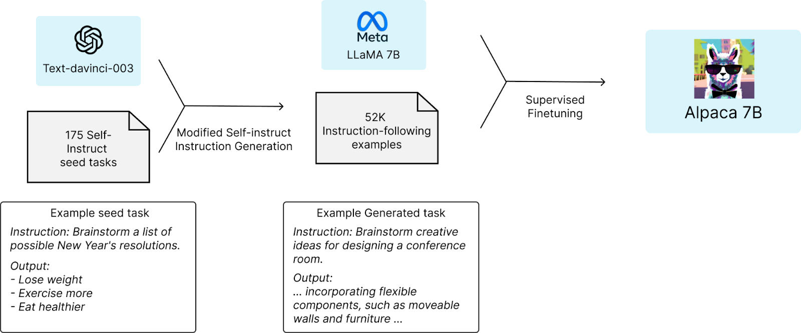
As a result, Alpaca became much better at following instructions than LLaMA 7B ever had been. Note that the dataset size is again not huge, it’s just 52K example even though this time manual labeling was unnecessary.

The next step, the Vicuna model introduced by Berkeley researchers Chiang et al. (2023), followed suit by training on 70K user conversations with ChatGPT. Vicuna-13B achieved over 90% response quality against ChatGPT (compared to 68% for basic LLaMA-13B and 76% for Alpaca-13B) while using a far smaller modthe training cost for fine-tuning was only about $300. 

There are many more examples of distillation (see also a survey of synthetic data for LLMs by Liu et al., 2024); important public datasets include:

• Orca (Mukherjee et al., 2022) and Orca 2 (Mitra et al., 2023), datasets distilled from GPT-4 to make lightweight models better, especially in logical reasoning and choosing a viable strategy for answering a question;
• Unnatural Instructions (Honovich et al., 2023), a dataset based on Super-Natural Instructions that we have discussed above (Wang et al., 2022); to create synthetic data, the authors take three examples from Super-Natural Instructions as few-shot instructions and ask a strong LLM to generate the fourth;
• Baize (Conover et al., 2023), a corpus of multi-turn conversations generated with ChatGPT and used to fine-tune the Dolly model we have discussed above;
• and lots and lots of domain-specific datasets such as, e.g, WizardCoder (Luo et al., 2024), WaveCoder (Yu et al., 2023), and Magicoder (Wei et al., 2023) for programming, that is, source code generation, WizardMath (Luo et al., 2023), MetaMath (Yu et al., 2023), and Xwin-Math (Li et al., 2024) for mathematics, and so on.

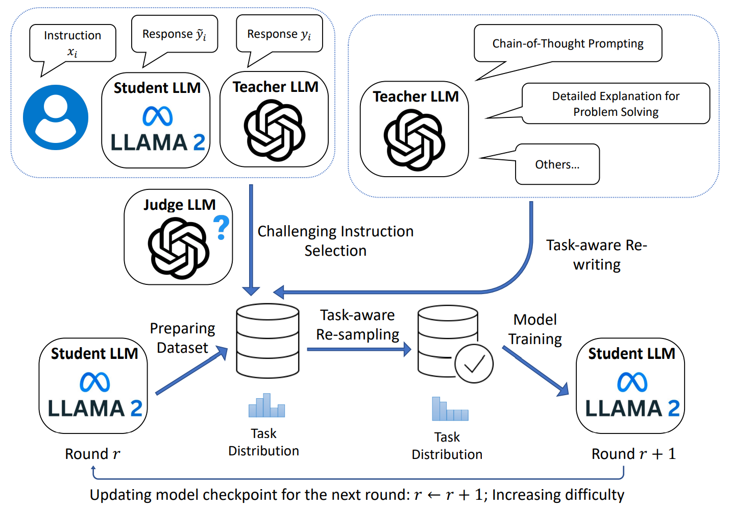
In an interesting recent work, Yue et al. (2024) note the importance of the task distribution inside the fine-tuning dataset, both in terms of difficulty and actual composition of tasks. They propose Task-Aware Curriculum Planning for Instruction Refinement (TAPIR), a multi-round framework that provides the student LLM with problems of increasing difficulty and balanced task distribution:

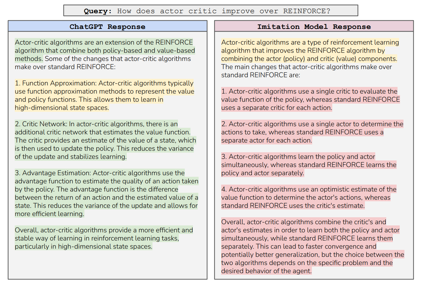
The results of distillation efforts may look too good to be true: you take a model with 7B or 13B parameters and achieve results virtually on par with a 100B+ teacher model. There is criticism that suggests that it is indeed too good to be true: UC Berkeley researchers Gudibande et al. (2023) studied the outputs of fine-tuned LLMs more closely and found that while the smaller models learn to imitate the style of larger ones almost perfectly, the actual content is far more often incorrect and prone to hallucinations. Here is an example from their work (conveniently explaining an important notion from one of our previous posts) where the response styles are identical but the explanations of the imitation model are just… totally wrong:

But be it in style or in substance, the distillation approach from “teacher” to “student” will never give you a model stronger than the teacher; this is a way to get smaller models up to speed with larger ones, not push the frontier. In a different direction of using synthetic data for LLM fine-tuning, researchers are finding ways to bootstrap already strong models into something even better by using the model’s own outputs as synthetic training data. 

Bootstrapping and Self-Improvement for LLMs

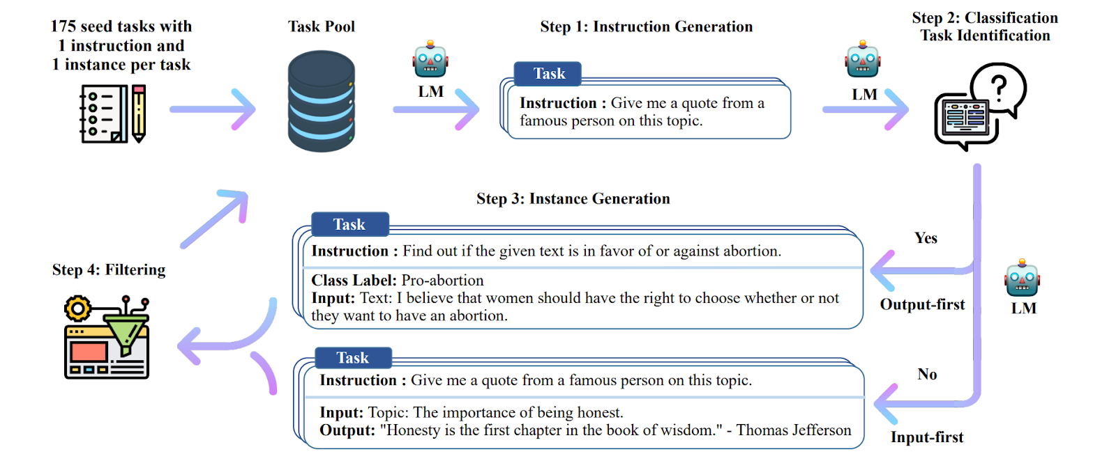
The archetypal work in this direction is the Self-Instruct pipeline presented by Wang et al. (2023). They begin with a “vanilla” LLM, in this case GPT-3, and a relatively small set of manually written tasks (175 tasks with only one sample instance per task) that serve as a seed for further generation. Then the process goes as follows:

• ask the LLM to generate new instructions with a few-shot prompt; Wang et al. show 6 human-written instructions and 2 previously produced model-written instructions as examples and ask for a new one;
• identify whether the result is a classification task; this is also achieved with a few-shot prompt to the same LLM;
• given the instructions (including newly generated ones), ask the LLM to generate novel instances for them, either input-first (generate an input, then generate a response) or output-first (begin with generating the response and then ask for a matching input);
• apply some straightforward filtering that promotes diversity across tasks and instances;
• when you have collected enough tasks and instances, fine-tune the LLM with this dataset; Wang et al. generated about 52K instructions and 82K instances for them before fine-tuning.

Here is the general pipeline as illustrated by Wang et al. (2023):

As a result, the Self-Instruct pipeline raised a basic vanilla GPT-3 almost to the level of InstructGPT, with no manual labeling or other human work beyond the original 175 task instructions.

A natural extension that the Self-Instruct paper (suspiciously) omits would be to take the fine-tuned model and re-apply the bootstrapping pipeline recursively. There will be limits to improvements, of course, but how good can you make a model in this direction? Recursive self-improvement of LLMs is partly the stuff of AI doomer nightmares (see, e.g., our previous post on the dangers of AGI) but at the same time it is already happening in practice! This brings us back to reinforcement learning.

In RLHF, you collect new data by evaluating LLM responses as you go; note that in principle you could straightforwardly make RLHF into a bootstrapping self-improvement mechanism by delegating evaluation to the same LLM. Several important works extend and improve the basic idea of RLHF by combining it with offline training on collected data.

In particular, DeepMind researchers Gulcehre et al. (2023) introduce Reinforced Self-Training (ReST), a pipeline where the current policy generates a dataset on the “Grow” step, and then the policy is updated by fine-tuning on the “Improve” step:

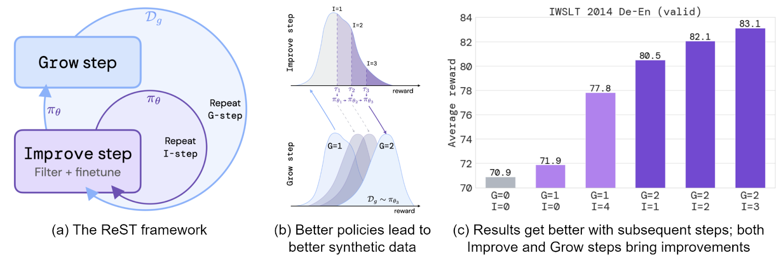
This is basically an application of offline reinforcement learning (Levine et al., 2020) to LLMs, and Gulcehre et al. (2023) report significant improvements; their paper shows results in machine translation, but, of course, a similar framework could be applied to any set of tasks.

Recursive self-improvement for LLMs lies in the center of DeepMind’s attention; it’s only natural for a company that brought us such RL-based marvels as AlphaGo, AlphaZero, MuZero, AlphaStar, and the AlphaFold series. In another recent work, DeepMind researchers Singh et al. (2024) further improve the ReST framework with ideas based on the expectation-maximization algorithm (EM). It is a rare opportunity for me to take a detour into the probabilistic side of machine learning, so let me explain expectation-maximization in a bit more detail (I actually wrote “delve into” at first but edited it out lest you think I’ve been delegating these posts to LLMs – what a world we live in!).

In general, the EM algorithm is intended for situations where we have a simple model of the data, but some of the variables in this model are latent, i.e., unknown. The prototypical example is clustering: it usually presumes a really simple model of each cluster (a Gaussian distribution, for example) but it is not known which points belong to which cluster. In general, given a dataset X = {x₁,…,x_N}, we want to maximize its likelihood

But this problem is intractable as written because p(x|θ) is a complicated model (a mixture of Gaussians, for instance), and to get back to a simpler model you need to know some latent variable z for every x. If we knew which cluster every point belongs to (that’s the z variable), learning a clustering model would reduce to learning the parameters of several individual Gaussians, which would be trivial. In general, EM is useful if p(x, z|θ) is simple but p(x|θ) is hard.

The EM algorithm in this case finds a lower bound for the log likelihood, log p(θ|X), that would be actually tractable; maximizing the lower bound turns out to be equivalent to maximizing

Note how here we are no longer talking about the complicated distribution p(X|θ) but only about the much simpler distribution p(X, Z|θ); this is the main goal here. The expectation looks complicated but in most actual cases, it just boils down to computing the expected values of the z variables under the previous model θ⁽ⁿ⁾. So while formally the EM algorithm is just repeating the single step of maximizing Q(θ, θ⁽ⁿ⁾) and repeating with the new θ⁽ⁿ⁺¹⁾ until convergence, in reality this maximization usually breaks down into two separate steps that gave the algorithm its name:

• on the expectation step, the algorithm computes the expectations of latent variables E[z];
• on the maximization step, it substitutes these expectations into log p(X, Z|θ) and maximizes the result with respect to θ; then the procedure is repeated with the new value of θ until convergence.

This post is not the time or place to provide a full explanation of why Q is a lower bound or how EM works in general, but if you smell something similar to variational approximations that we discussed some time ago, you are completely correct.

In practice, the EM algorithm often simply means taking the expectation of whatever makes the problem intractable and plugging it into the model (although you do need to check that it makes sense in each specific case). For LLMs, we are trying to optimize some metric (reward) over the possible outputs of a language model. The objective function is thus an expectation over LLM outputs, and of course it would be intractable to take the sum over all possible sequences of tokens. This is where the EM algorithm comes into play:

• the expectation step turns out to be weighting the output samples according to the probability of obtaining high rewards;
• and then you can fine-tune the LLM with an objective function weighted by these probabilities.

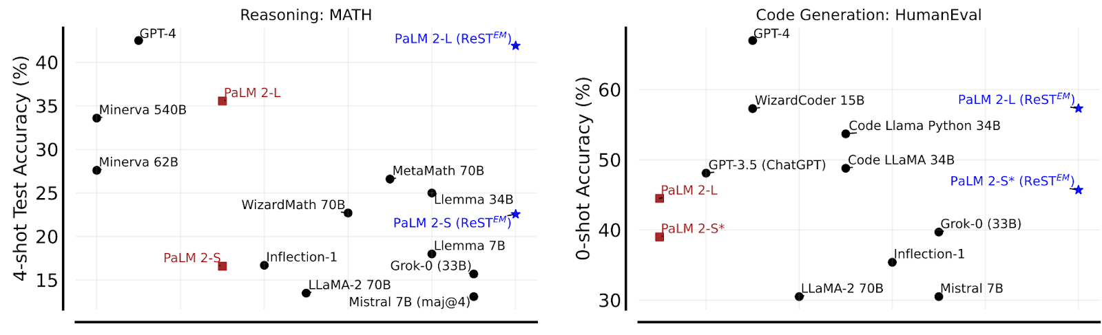
Singh et al. (2024) apply this framework to large-scale models from the PaLM family and actually achieve great results in two chosen tasks, mathematical reasoning and code generation (the X-axis shows approximate release time):

And here are the plots showing how EM iterations help for these problems:

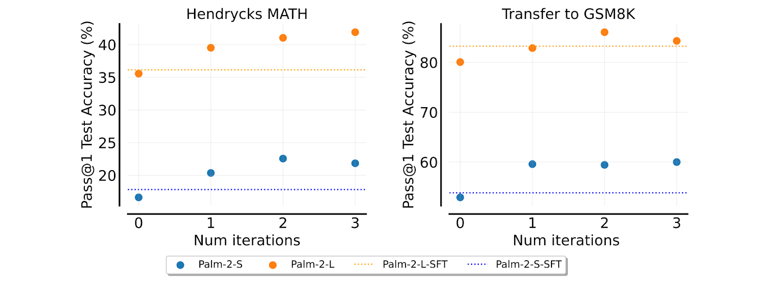
Interestingly, the models fine-tuned on synthetic data with several EM iterations clearly outperform the same models fine-tuned on human-labeled data (shown with dotted lines on the graphs)! Note that GPT-4 still comes out on top, so we are not yet talking about pushing the actual frontier, but the approach looks very promising.

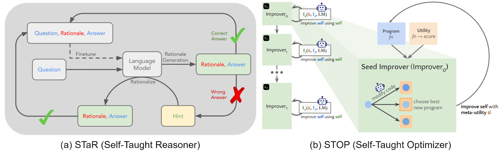
DeepMind seems to be leading the way; tweets like this one definitely make you wonder what else they have in stock. But there are other efforts in (usually RL-based) recursive self-improvement for LLMs. In particular:

• Self-Taught Reasoner (STAR; Zelikman et al., 2022) bootstraps rationale generation, i.e., generating explanations such as the ones that an LLM would produce when asked to “reason step by step”; the authors ask the LLM to produce a lot of rationales, filter the ones that lead to the correct answer, and then fine-tune the LLM on the filtered dataset (shown on the left in the figure below);
• Rejection Fine-Tuning (RFT; Yuan et al., 2023) takes this idea one step further, developing a better filter for reasoning paths (they specialize in mathematical reasoning, so reasoning paths are chains of equations in this case) based on rejection sampling, looking for the most diverse paths to improve reasoning; moreover, they find a log-linear dependence between the amount of data and model performance and show how better data (e.g., filtered with RFT) can lead to better models;
• Self-Taught Optimizer (STOP; Zelikman et al., 2024) takes another meta-step: it recursively improves the code (here, the application is coding) that is designed to apply a language model to improve a source code solution for an arbitrary problem; that is, the improver program is called on itself, and the “improved improver” actually generates better programs for downstream tasks (shown on the right in the figure below).

Overall, I think recursive self-improvement approaches hold a lot of promise even if they don’t achieve the actual fast takeoff singularity (do we really want to achieve that?). The story of machine learning in many different domains comes to the same conclusion: you can succeed up to a point when you try to imitate humans, and LLMs are the best example of this. But if you want to achieve superhuman capabilities, you really need to find a way of recursive self-improvement. In chess and Go, decades of trying to emulate the patterns of human thinking led to some breakthroughs, but when AlphaZero is learning from scratch it just breezes through the top human level without even noticing it, the saturation point comes much later.

So far, LLMs are mostly trained to imitate human reasoning; after all, the main training process is done on texts written by humans. Can we find a way to bootstrap the model and breeze through the imperfections of human-generated data? Maybe not in general problem solving anytime soon, but at least in more formalized domains such as coding and math where it is easier to generate synthetic problems? Time will tell, and I’m really not sure how much time we are talking about here.

Conclusion

In this post, we have discussed the main directions of making language models better. We have seen how a pure token prediction machine can become more helpful and/or more specialized via various forms of fine-tuning or adapter training.

There are other approaches, too. For instance, we have not mentioned RAG, retrieval-augmented generation, where the generator model is supplemented with an information retrieval mechanism able to gather important information from separately provided sources (Lewis et al., 2020). RAGs are also very important for modern LLMs, but this will be a story for another day. We also did not mention tricks that make training and/or fine-tuning more efficient, such as mixed precision training or gradient checkpointing, which do not provide new ways to adapt models but may significantly extend the feasibility of existing approaches. Finally, another important story is how to best extract the knowledge and reasoning abilities that are already contained in the models, even without any fine-tuning. This is the subject of the rapidly growing field of prompt engineering, a field that already goes far beyond the “please reason step by step” trick (although it is still surprisingly effective).

Next time, we will discuss another important aspect of the journey that modern generative AI has made over the last couple of years; stay tuned!

Sergey Nikolenko
Head of AI, Synthesis AI