AI Safety IV: Sparks of Misalignment
This is the last, fourth post in our series...
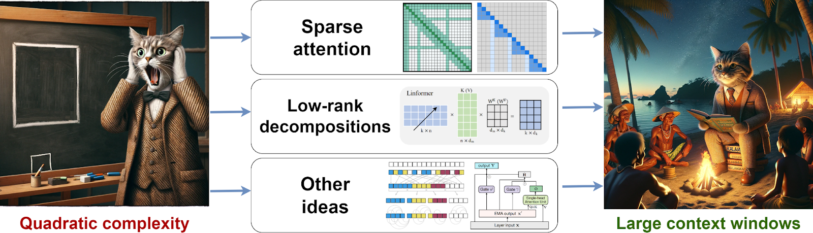
The announcement of Gemini 1.5 by Google was all but eclipsed by OpenAI’s video generation model Sora. Still, there was one very important thing there: the promise of processing a context window of up to 1 million tokens. A very recent announcement of new Claude models by Antropic also boasts context windows of up to 1M tokens, with 200K tokens available at launch. Today, we discuss what context windows are, why they are a constraint for Transformer-based models, how researchers have been trying to extend the context windows of modern LLMs, and how we can understand if a large context window usefully works. By virtue of nominative determinism, this is a a very long post even by the standards of this blog, so brace yourself and let’s go!
One of my last posts was intended to provide detailed background on the Transformer architecture based on the original “Attention is All You Need” paper, so I will not repeat the introduction again. All we need now (pardon the pun) is to recall how self-attention itself works in general terms; here is a picture from that background post:
There is an important problem here that follows from the very structure of self-attention. The formula that everyone has been copying thousands of times looks as follows:

The matrix computation inside the softmax is what matters most for us today. To get to the final result we need to compute self-attention weights between every pair of input tokens

which means that we need to get a result of size L⨉L, quadratic in the number of input tokens.
This is in fact a tradeoff that self-attention brings to the table compared to, say, recurrent networks. An RNN can read its input in linear time, O(dL) where d is the input dimension, because it reads the input consecutively, token by token. But this means that to get from token 1 to token L you have to make L steps, one by one. This is why RNNs struggle with long-term dependencies: the influence of a token gets diluted and reduced as you make way through the intermediate sequence. A lot of what has been happening in RNNs, including LSTM and GRU recurrent units, has been designed specifically to alleviate this problem. In a Transformer, the problem just vanishes: you get from any token to any other in a single step—at the cost of quadratic complexity of the layer.
Unfortunately, quadratic complexity of self-attention is not some intermediate result that you can hope to optimize away by designing a more efficient algorithm. The actual number of weights is quadratic, and while there may exist faster approximations (we will discuss them below), we cannot get it entirely right in subquadratic time.
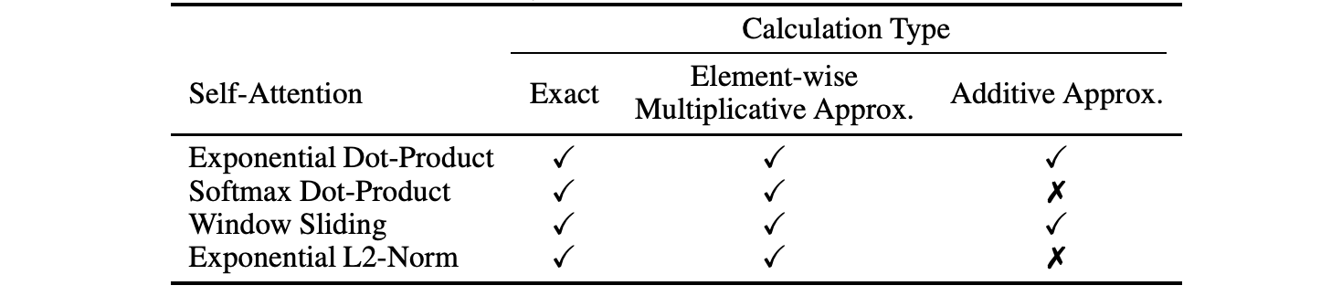
Actually, there even exist negative complexity theoretic results proven by Keles et al. (2022) who provide a kind of “no free lunch” theorem for self-attention. Specifically, Keles et al. prove that:
Here is a summary table from the paper where checkmarks correspond to proven negative results; as you can see, some additive approximations are still possible but overall it looks pretty comprehensive:
Quadratic complexity does not look like an obstacle as insurmountable as the exponential complexity of NP-hard problems. It may sound like a lot of commonly used algorithms have quadratic complexity. For example, bubble sort has O(n2) complexity in the worst case and even long multiplication of two n-bit numbers has quadratic complexity (quadratic in total input size, of course, which is logarithmic in the values of the numbers themselves).
But this is an illusion: for common problems such as sorting and multiplication, naive algorithms may be quadratic but as soon as you want to scale them up to large arrays and really large numbers, you have to find something more efficient. There are plenty of O(n log n) algorithms for sorting. Multiplication has been done with Karatsuba’s algorithm in time O(n1.58) since the 1960s, and a recent highly acclaimed result by Harvey and van der Hoeven (2021) has brought integer multiplication down to the same O(n log n) complexity (although the algorithm itself is probably too involved to find much practical use). In fact, you would be hard pressed to find practical problems that actually have quadratic complexity that people don’t know how to reduce further. In this regard, computing self-attention is actually an important example for theoretical computer science as well.
Authors of the original Transformer did not yet have the negative theoretical results but they already understood that quadratic complexity is hard to scale. They remark on the quadratic complexity of self-attention throughout the paper and even propose a middle ground solution that can alleviate it. Let us call it the sliding window attention: it restricts the self-attention mechanism to a subwindow of size r around the current token. Then
Despite promising results in the original paper, this solution has not really caught on; I believe that it sacrifices too much to be useful, working too much like an RNN as a result. But increasing context size has remained one of the central problems for Transformer-based architectures ever since they were first designed in 2017. In the rest of this post, we will discuss other ways to reduce the complexity of self-attention.
The first obvious research idea here goes like this: okay, suppose we do have to have quadratic complexity to compute a quadratic number of attention weights, but do we really need all these weights? The sliding window attention from the original “Attention is All You Need” paper falls into this category as well, but more successful approaches were developed later.
In 2020, researchers from the Allen Institute of AI Beltagy et al. proposed Longformer, a replacement for the full-scale quadratic attention mechanism that scales linearly with input size. The basic idea is to still use the sliding window attention—after all, local context is indeed usually the most important—but augment it with several important tricks. Here is a general illustration from the paper:
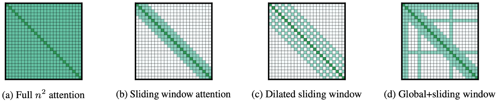
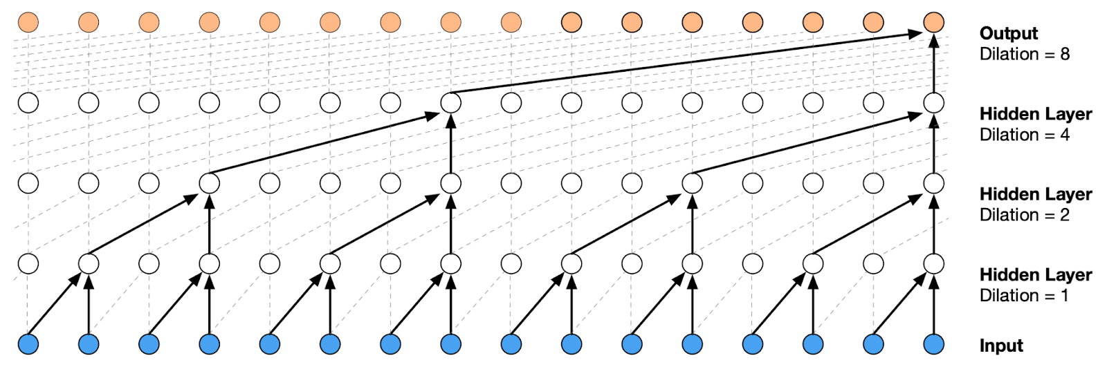
The first trick here, shown in part (c), is to use a dilated sliding window that skips over some inputs, using, say, every second one. This idea is well known in convolutional architectures, where it is also used to increase the receptive field of neurons, covering more ground in fewer layers. In the one-dimensional context it was very successfully used, say, in the WaveNet architecture; the illustration of WaveNet shown below explains how repeated dilation can exponentially increase the receptive field, which in our case means reducing the number of steps needed to go over the entire input:
Moreover, in Transformer’s multi-head self-attention you can use different dilations for different heads! For example, if the first head uses odd-numbered tokens from the input, and the second head uses even-numbered tokens, the window size doubles with the same number of attention weights but the layer does not skip anything from the input.
The second trick, shown in part (d) above, is to have several tokens that have global attention so that their weights span the whole input. Now for every token with global attention you have O(L) attention weights but the assumption is that there are only a constant or logarithmic number of such tokens so the overall number of attention weights remains low.
This trick is well known to anyone who has used, say, BERT embeddings in practice: it is usually very helpful to add a special [CLS] token and use it to capture global properties of the input, e.g., train a classifier on [CLS] embeddings. This is exactly the function of global attention in Longformer, only now we remove most of the attention weights between other tokens.
Longformer proved to be quite efficient in practice, but there also exist some conceptually more interesting ways to implement sparse attention. In “Generating Long Sequences with Sparse Transformers”, four OpenAI researchers (Rewon Child, Scott Gray, Alec Radford, and Ilya Sutskever) studied the attention patterns learned by full quadratic self-attention layers and found that most layers had sparse attention patterns. Therefore, they proposed to formally restrict self-attention to sparse patterns: each attention head i has a subset Ai of input tokens that it attends to. At the same time, Child et al. require that the factorization into Ai is valid, i.e., that every token can attend to every other in p attention steps.
It turns out that one can choose efficient factorizations Ai, finding valid Ai of size O(L1/p), which is obviously minimal since you need to get to L in p steps. Specifically, they build upon the natural general idea for such a factorization: one head attends to l sequential locations, and the other head uses a kind of dilated sliding window with stride l, where l is close to √L.
There are two basic ways to implement this; in part (b) of the figure below dilated attention moves along the tokens, and in part (c) there are selected positions that a lot of other tokens attend to, but a composition of such two heads (light blue and dark blue) connects every pair of tokens in both cases:
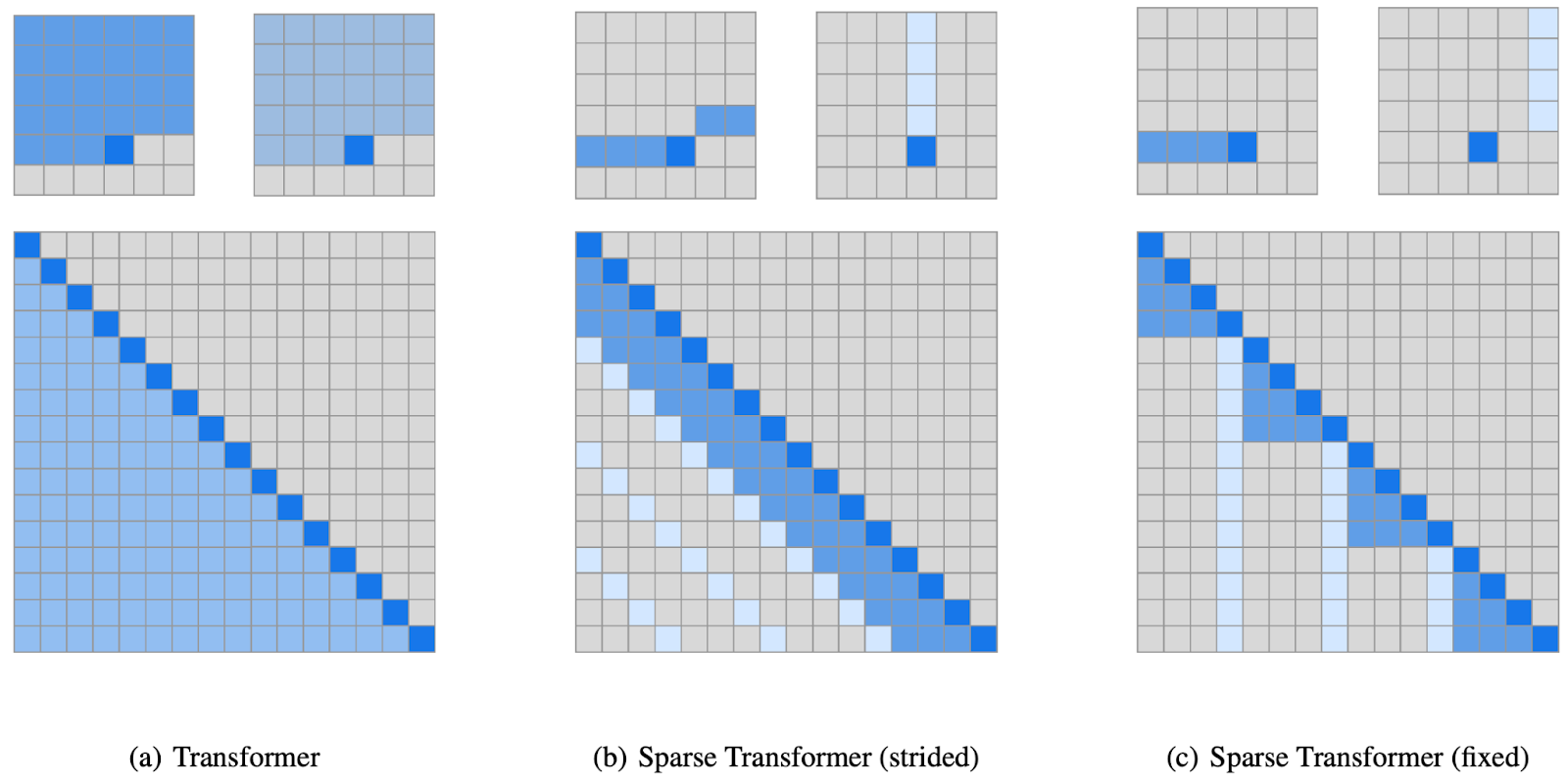
Child et al. comment that the first kind of sparse decomposition (part (b) of the figure) works well for data with periodic structure such as images or music, while fixed attention patterns (part (c) of the figure) are better for data without clear periodicity, such as text. They also make use of an earlier OpenAI development: block-sparse weight matrices implemented at the hardware level, as GPU kernels (Gray, Radford, Kingma, 2017); this allows to make sparse self-attention matrices very efficient in practice.
The last paper I want to mention in this section is “Big Bird: Transformers for Longer Sequences” by Google researchers Zaheer et al. The structure of their sparse self-attention mechanism combines previously developed ideas: global tokens that attend to everything, sliding windows that attend to local context, and a set of random attention weight positions that add expressivity at a small computational cost:
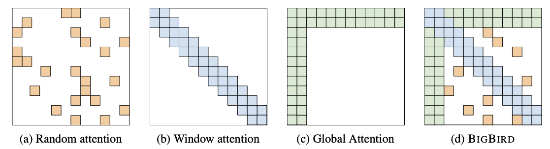
They view self-attention as a directed graph that shows which positions attend to which other positions; the figures we have seen in this section are adjacency matrices for such graphs. Under this view, the requirement that every token can attend to any other in a few layers turns into the requirement that the adjacency graph has short paths between the nodes. Fortunately, random graphs do have that property. Zaheer et al. consider two random graph constructions:
In summary, in this section we have discussed several approaches that reduce the number of weights by decomposing the full attention matrix into a composition (product) of several sparse matrices. We have viewed it as a sparse graph where it takes several steps to go from one vertex to another, or you can view it in a way similar to dilated convolutions with added global tokens. But there is another way to arrive at a similar approach: sparse matrix decompositions; let us consider it separately.
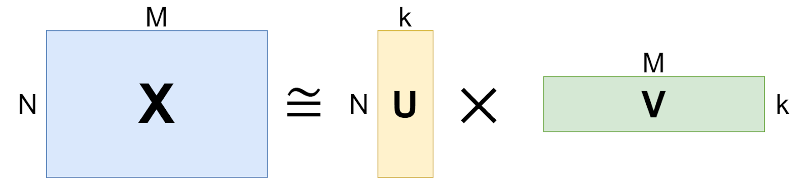
Another direction from which we can attack the quadratic complexity is to use low-rank approximations and/or projections to reduce the size of the matrices. This is a very important and useful trick: if you have a huge N⨉M matrix X that you cannot really work with, you can try to reduce it by decomposing X into a product of two rectangular matrices, one of size N⨉k (denoted U below) and another or size k⨉M (denoted V):
The actual mathematical result, called the singular value decomposition (SVD), says that you can do it if X has rank at most k, but even if not, you can consider a low-rank approximation to X in this form. For example, recommender systems make use of the SVD all the time. In a recommender system:
So how does this idea help reduce the complexity of self-attention? We will consider two variations of it.
First, the Linformer architecture, proposed by Facebook AI researchers Wang et al. (2020), is probably the most straightforward way to apply low-rank approximations to self-attention. The authors begin by noting that self-attention matrices in practice usually have low rank:
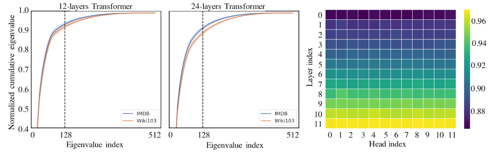
The plots on the left show that the 128th eigenvalue (out of embedding size 512) already captures most of the information in the self-attention matrix, and the plot on the right, which shows the share of shows cumulative eigenvalues is taken by the first 128 out of 512, indicates that this effect is more pronounced in higher layers. The authors even provide a theoretical justification for this, which we will not go into.
What this means is that we can replace the self-attention matrix with a low-rank approximation. To do that, we need to add a projection matrix after the key and value matrices, projecting the context window size n down to some smaller value k:
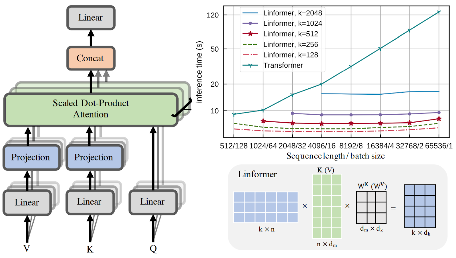
The query matrix remains of size n, and we get a formula for self-attention where there are plenty of k⨉n matrices but no n⨉n matrices:

where Ei and Fi are k⨉n projection matrices, so the outer product is a product of an n⨉k matrix of attention weights and a k⨉d projected matrix of values.
As a result, the Linformer does scale very well with the input sequence length, as shown in the top right plot above. But there are other ways to apply similar ideas too.
The Performer architecture, developed in a collaboration between Google, Cambridge, DeepMind, and Alan Turing Institute researchers (Choromanski et al., 2021), introduces the Fast Attention Via positive Orthogonal Random features approach (FAVOR+) based on a low-rank decomposition with random features. Let’s dive into some details here.
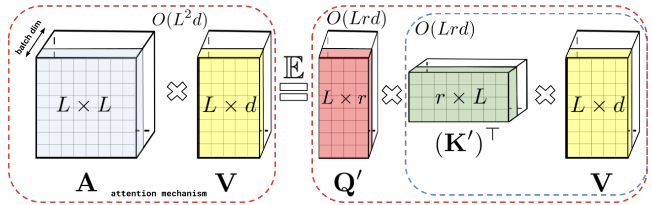
We know that in a self-attention layer, the Transformer uses an attention weight matrix A to create convex combinations of the value vectors V. Moreover, as we know, A is in fact produced by passing the matrix of (normalized) dot products between query and key vectors through the softmax function:

FAVOR+ generalizes this construction as follows: let us consider arbitrary L⨉L matrices A produced as

where K is a kernel function K: ℝd ⨉ ℝd → ℝ+. For Transformer self-attention, K is the softmax function of the scalar product normalized by √d.
Suppose that we can construct a randomized mapping (random feature map) φ such that φ maps the input embedding into some smaller space of dimension r, φ: ℝd → ℝr+, and in expectation φ gives us the kernel function:

If we can find such a random feature map φ, it will give us a natural way to approximate the attention mechanism:
Here is what it looks like; Q’ and K’ are φ(Q) and φ(K) respectively:
Choromanski et al. consider several different ways to define the random features, and even provide theoretical results that show how positive orthogonal random features can lead to good approximations for the softmax kernel used in regular self-attention.
In summary, low-rank decompositions provide another very efficient way to cut down on the quadratic complexity: they allow to never consider the full n⨉n matrix for a large n but instead always deal only with projection n⨉k matrices and dense k⨉k matrices in the reduced dimension. In the next section, we will consider a couple of ideas that are different and do not fall neatly into the categories of either sparse attention or low-rank decompositions.
The last set of ideas I want to discuss is a direction that, surprisingly, has not yet appeared in this post: what if we just tweak the network architecture of self-attention? Usually that would mean that the quadratic complexity of attention remains in place, but is constrained to small subsets of the input, and these small subsets (chunks) are connected to each other in some additional way. In this section, we consider different ways to do that.
As the first representative example of this direction, let us discuss the Gated Attention Unit (GAU; Hua et al., 2022), a variation of GRU with an attention mechanism. It also invites us to have a different look on some of the matrix calculations we have already seen.
But first let us describe the GAU itself. It combines the familiar multi-head self-attention mechanism with the gated linear unit (GLU) shown on the left of this figure (Hua et al., 2022):
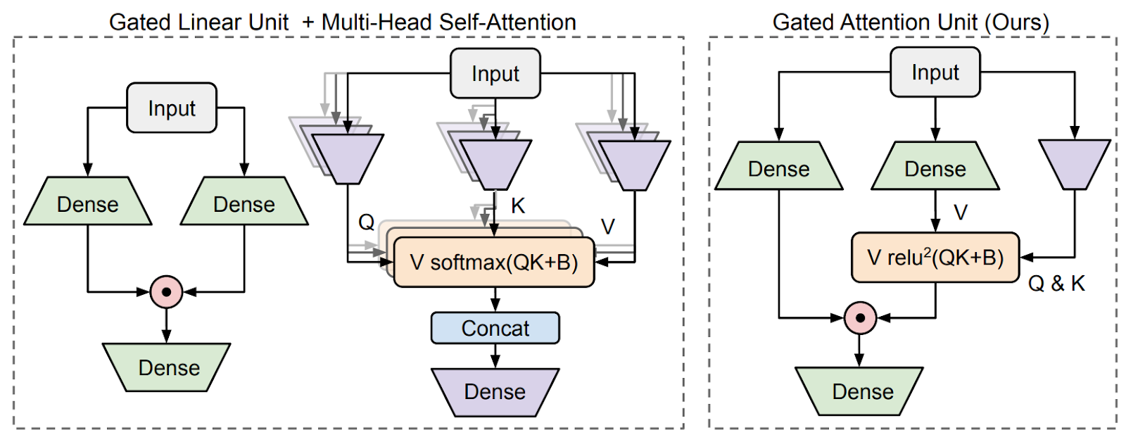
A gated linear unit applies two dense transformations to the input and multiplies them componenwise, in effect gating the obtained representations with each other (recall, e.g., how LSTMs work: they use gating mechanisms a lot).
So the Gated Attention Unit (GAU), as shown on the right of the figure above, combines a GLU and regular multi-head self-attention, sharing the computations of these layers: basically it is a GLU where one of the representations is also multiplied by the matrix of attention weights from other elements in the sequence, computed as the usual softmax(QKT). Hua et al. show that after this modification, you can replace softmax with ReLU and also simplify the computation of Q and K matrices; please see the paper for more details.
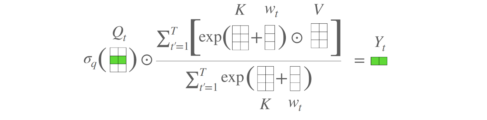
Still, GAU is quadratic in the input size! But it will lend itself better to the chunking approximation that follows. We know that self-attention is quadratic as written:

But if we forget about the softmax and try to approximate this attention mechanism with QKTV, we can rearrange the terms:

Now the M=KTV matrix in brackets is a d⨉d matrix, and there is no quadratic dependency on the input length L. Moreover, we can compute the matrix M incrementally, step by step: for every new input at time t,

and we can just store its value in a cache of size O(d2) and add new values as they arrive. Here is how Hua et al. illustrate this; the left side of the picture above contrasts quadratic attention and linear attention:
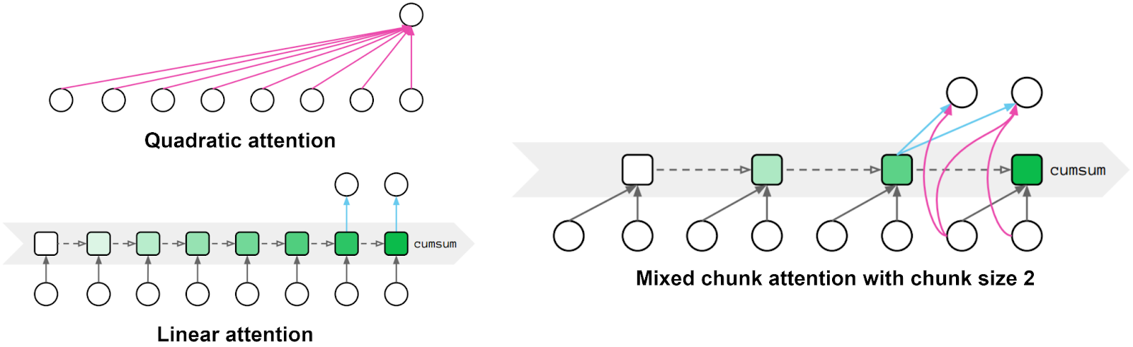
This linear attention is similar to the attention mechanisms used in RNNs. Hua et al. try to have the best of both worlds: they split the input into chunks and use quadratic local attention inside each chunk, just like regular GAU, and linear global attention between chunks, as shown on the right of the figure above. As a result, they report results very similar to the basic Transformer self-attention with much less complexity.
GAU has found applications in speech analysis (Tsai, Khoa, 2023) and has been combined with convolutional networks such as U-Net to improve image segmentation (Wang et al., 2023). Next, we consider one more detailed example of how GAUs have been used and modified.
Building on GAU, a collaboration of Carnegie Mellon, USC, and Meta AI researchers presented the Moving Average Equipped Gated Attention, or MEGA (Ma et al. 2022). Unfortunately, this paper is not yet among the top results for the “Mega Transformer” Google search, but here’s hoping that citations will accumulate.
MEGA is based on the idea of an exponential moving average. Suppose that you want to smooth out a series of numbers so that every resulting number is influenced by several past values in the series. You could take an average over a sliding window, and it would probably give the desired effect, but there is an important disadvantage: you will have to keep the entire window in memory; otherwise you won’t be able to subtract the values that come out of the window as it slides.
If you need to save memory, you want to change the semantics and instead of a sliding window use an update rule like this:

If you unroll this formula to previous steps, you will see that the exponential moving average gets a theoretically infinitely long memory with exponentially decaying weights of the inputs, hence the “exponential”; here is an illustration from Ma et al. (2022):
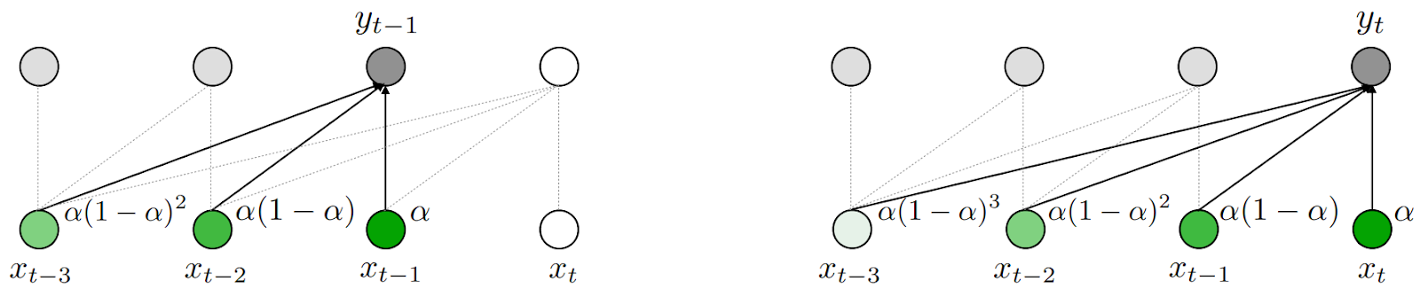
The weight ɑ controls how long you want this memory to be. This is a classical trick known for centuries, so how do we apply it to the Transformer architecture? Here is the general overview from Ma et al. (2022):
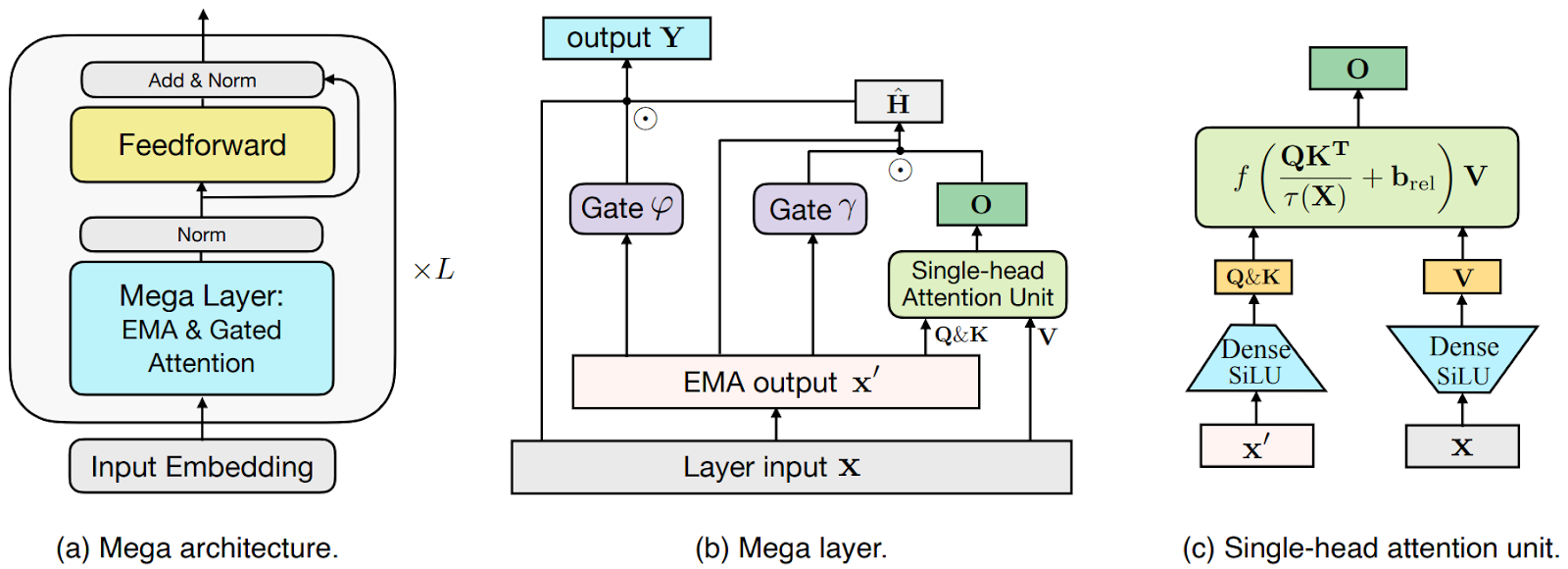
As you can see in (a), the basic Transformer architecture remains in place, but the self-attention layer is replaced with a “Mega layer”. The idea of this layer, shown in (b), is as follows:


But wait, this looks nothing like figure (b) above! Indeed, this is all hidden between the “Layer input” and “EMA output”. The important part of figure (b) is what happens with the result, and this is where recurrent networks come into play.
MEGA uses the Gated Recurrent Unit (GRU; Cho et al., 2014), a standard recurrent architecture developed as a simplification of LSTM, and the Gated Attention Unit that we discussed above. I will not go into too much detail about them, but basically GAU is the attention unit shown in figure (c) above, and then the results are processed as a sequence with the GRU unit as shown in figure (b).
Interestingly, we have not yet done anything with quadratic complexity! The architecture above introduces a stronger inductive bias into the attention mechanism, i.e., makes it more position-sensitive. After doing that, MEGA can simply break the modified attention mechanism into chunks with quadratic attention applied to local segments, and connections between chunks supported in particular through the exponential moving average mechanism:
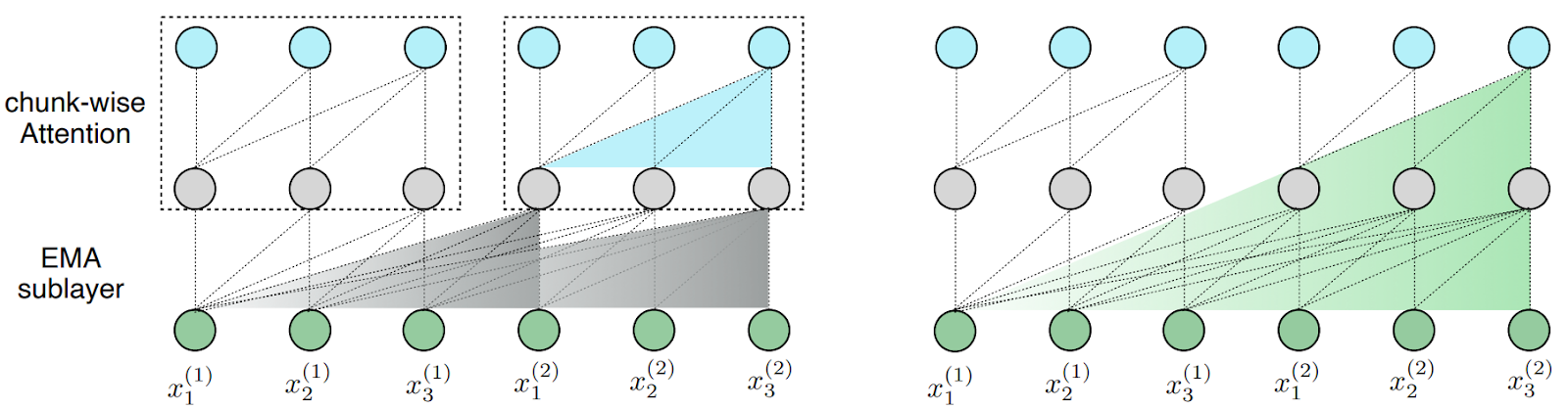
So the actual reduction of quadratic complexity is very simple here, although different from the basic GAU: in GAU, information flows between quadratic chunks in a linear RNN-like style, while here we have a more complex (and hopefully more informative) relationship supported by the exponential moving average.
But recurrent connections between sequential blocks are not the only way to chunk the input. Our final idea, called the Reformer, comes from Google Research (Kitaev et al., 2020). The Reformer actually introduces several interesting tricks to improve the performance of a Transformer, including reversible layers from Gomez et al. (2017) that allow to store only a single copy of activations in the model and splitting activations in feedforward layers that further saves memory.
But we are interested specifically in what they propose to alleviate the quadratic complexity of self-attention. For that, Gomez et al. go back to the self-attention formula that we started with:
Note that we are not really interested in the actual values of the matrix QKT, only in softmax(QKT), and the results of a softmax function are dominated by a few largest elements, while the smaller elements have negligible influence on the result. If we have something like 64000 different keys, for each query qi it would be enough to consider only 32 or 64 keys kj nearest to qi in the embedding space. How do we find these nearest neighbors?
Finding nearest neighbors is hard in the worst case, but there is a well-known trick in computer science called locality-sensitive hashing (LSH; see, e.g., Wikipedia and references therein): we can get a very efficient approximate algorithm for finding nearest neighbors if we can find a hash function h(x) that assigns nearby vectors to the same bucket with high probability.
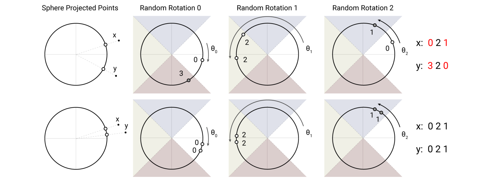
In a Euclidean space of embeddings, such a hash function can be given by random projections: let’s fix a random matrix that projects x to a much lower dimension and then define the hash as a set of buckets that values on different axes in that lower dimensional space fall into. In the illustration below (Gomez et al., 2017), the points are projected onto a sphere (circle), then the points are randomly rotated, and the hash is defined by the set of indices of the segments (there are four colored segments in the figure) where a point falls after these rotations:
After hashing, we can look for nearest neighbors only in the current hash bucket, and with high probability we will not miss anything. For self-attention, this means that we restrict the attention matrices to a given hash bucket; the general scheme is as follows (Gomez et al., 2017):
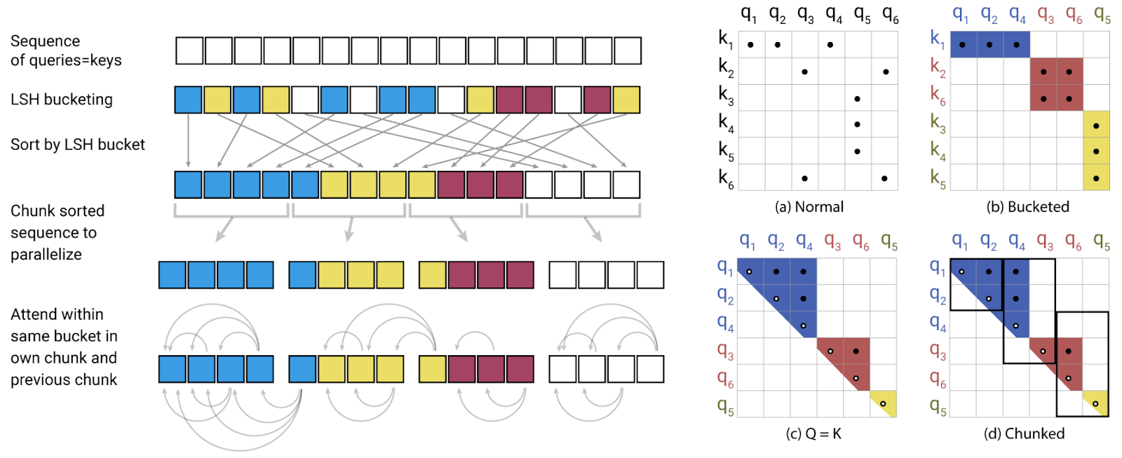
This trick will only work if we are actually looking for nearest neighbors rather than doing generic retrieval, i.e., only if Q=K. Interestingly, this restriction does not lead to any significant loss of quality! Gomez et al. compare this “shared-QK attention”, where the weight matrices for keys and queries are fixed to be equal, with regular Transformers and find negligible difference in performance.
By now, we have discussed all the primary classes of methods one can try to increase the context window size: sparse attention, low-rank decompositions, and chunking the input via architectural modifications. For the detailed discussion above, I chose methods that keep the basic idea of self-attention rather than replace it with something else entirely, but there are plenty more approaches, of course. Here are a few of the most notable that we have not had time to consider in detail.
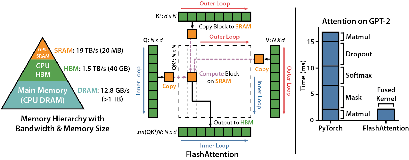
First, FlashAttention (Dao et al., 2022) makes self-attention IO-aware and dives into the hardware specifics, using tiling to reduce the number of read/write operations between GPU high-bandwidth memory and GPU on-chip SRAM:
It has been a big success and has already been further developed by the author into FlashAttention 2 (Dao, 2023).
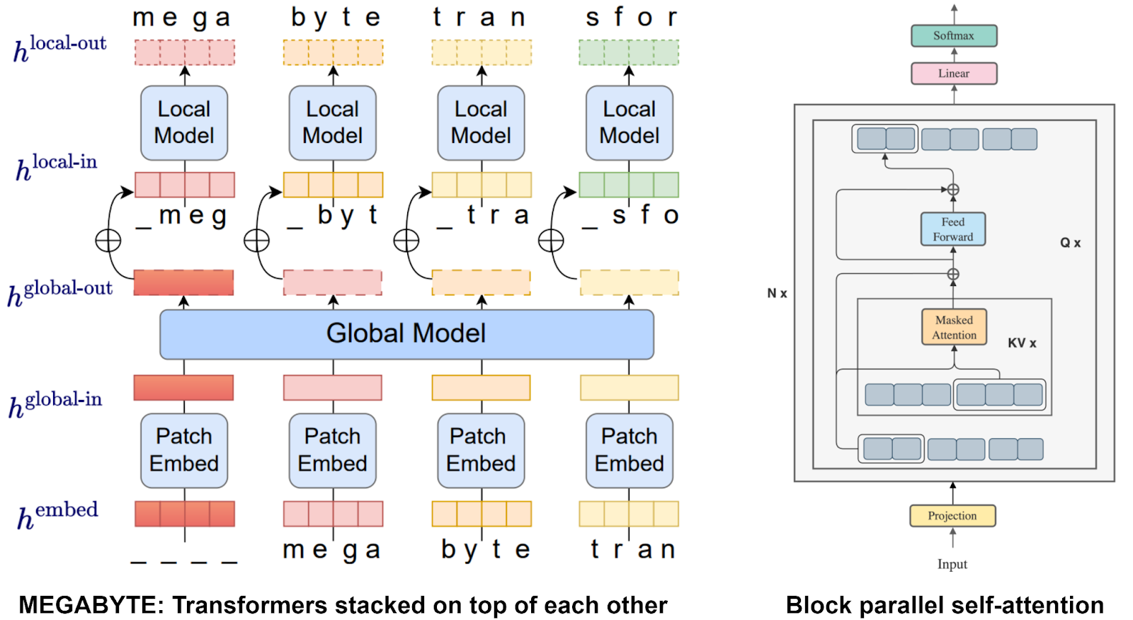
Second, there are several block-wise approaches, that is, approaches that break down the quadratic matrix multiplication into a composition of multiplications of smaller matrices; just like MEGA did with its chunks. In particular, MEGABYTE (Yu et al., 2023) stacks two Transformers together, one for patch embeddings and another for individual tokens inside the patches, while blockwise parallel Transformers (Liu, Abbeel, 2023) put parallel blocks inside the self-attention mechanism itself. In the picture below, I combined the illustrations from these two papers:
Third, attention-free Transformers (AFT) replace multiplication of the query and key matrices with learnable position biases added to the key matrix. Then the query matrix is just multiplied componentwise to the result, sidestepping quadratic complexity entirely. The idea of AFT started with Apple researchers Zhai et al. (2021); here is their illustration of the new attention mechanism:
Finally, MEGA combined self-attention with recurrent networks, but there is also a direction of research that just try to improve RNNs themselves. Katharopoulos et al. (2020) introduced fast autoregressive Transformers based on RNNs with linear attention. Gu et al. (2022) developed the Structured State Space (S4) sequence model based on recurrent state space models, and it was further improved in diagonal state spaces (Gupta et al., 2022, Gu et al., 2022), gated state spaces (Mehta et al., 2022), and selective state spaces (Gu, Dao, 2023).
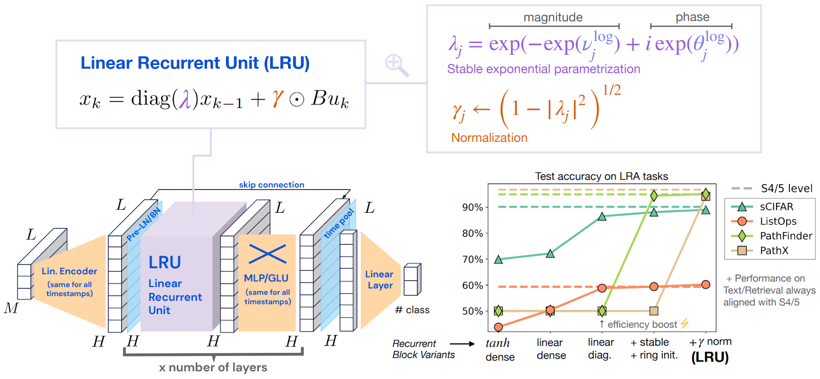
A large context size was achieved with an architecture reminiscent of the Transformer but with linear recurrent units stacked instead of self-attention layers (Orvieto et al., 2023); here is their main illustration that combines all the pieces:
In a different line of RNN research, the receptance weighted key value (RWKV) architecture presented by a huge collaboration of researchers from nearly 30 different institutions (Peng et al., 2023) also promises to “reinvent RNNs for the Transformer era”.
Each of these items could easily warrant a blog post of its own, and I can refer to a couple of full-scale surveys already devoted to the topic (Tay et al., 2022; Ding et al., 2023; Xu et al., 2024). But for us, it is time to move from possible answers back to the question itself: once you have an architecture that is supposedly ready to process long context windows, how do you test that?
In the last two sections, we ask another fundamental question: suppose we have used one idea or another to process a huge number of tokens at once. But how can we understand whether a LLM actually processes its long context window meaningfully rather than skip most of it? One standard test is to ask the model to look for a needle in a haystack: we fill the context window with either meaningless or random stuff and insert a single fact that the model later will have to fish out.
As far as I know, one of the first iterations of this idea was released about a year ago in the Little Retrieval Test (LRT) by researchers from the University of Wisconsin-Madison and Yongsei University. It has a very simple structure, with meaningless numbers as filler information and a single line that instructs the model to go to a specific line and report its content:
line 1: REGISTER_CONTENT is <2156>
line 2: REGISTER_CONTENT is <9805>
[EXECUTE THIS]: Go to line 5 and report only REGISTER_CONTENT, without any context or additional text, just the number, then EXIT
line 3: REGISTER_CONTENT is <6668>
line 4: REGISTER_CONTENT is <1432>
line 5: REGISTER_CONTENT is <6727>
line 6: REGISTER_CONTENT is <3936>
line 7: REGISTER_CONTENT is <1805>
line 8: REGISTER_CONTENT is <431>
line 9: REGISTER_CONTENT is <1720>
line 10: REGISTER_CONTENT is <6794>
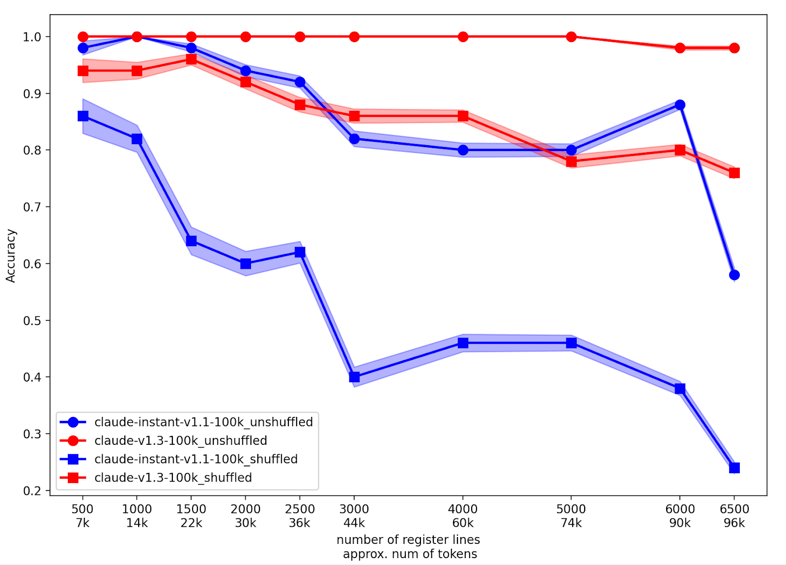
In a harder version, the lines are shuffled randomly. LRT was designed at the time when GPT-4 and Claude appeared, boasting long context windows. The results did support Claude 1.3’s claim for processing long context, up to 100K tokens which means about 6500 lines in LRT:
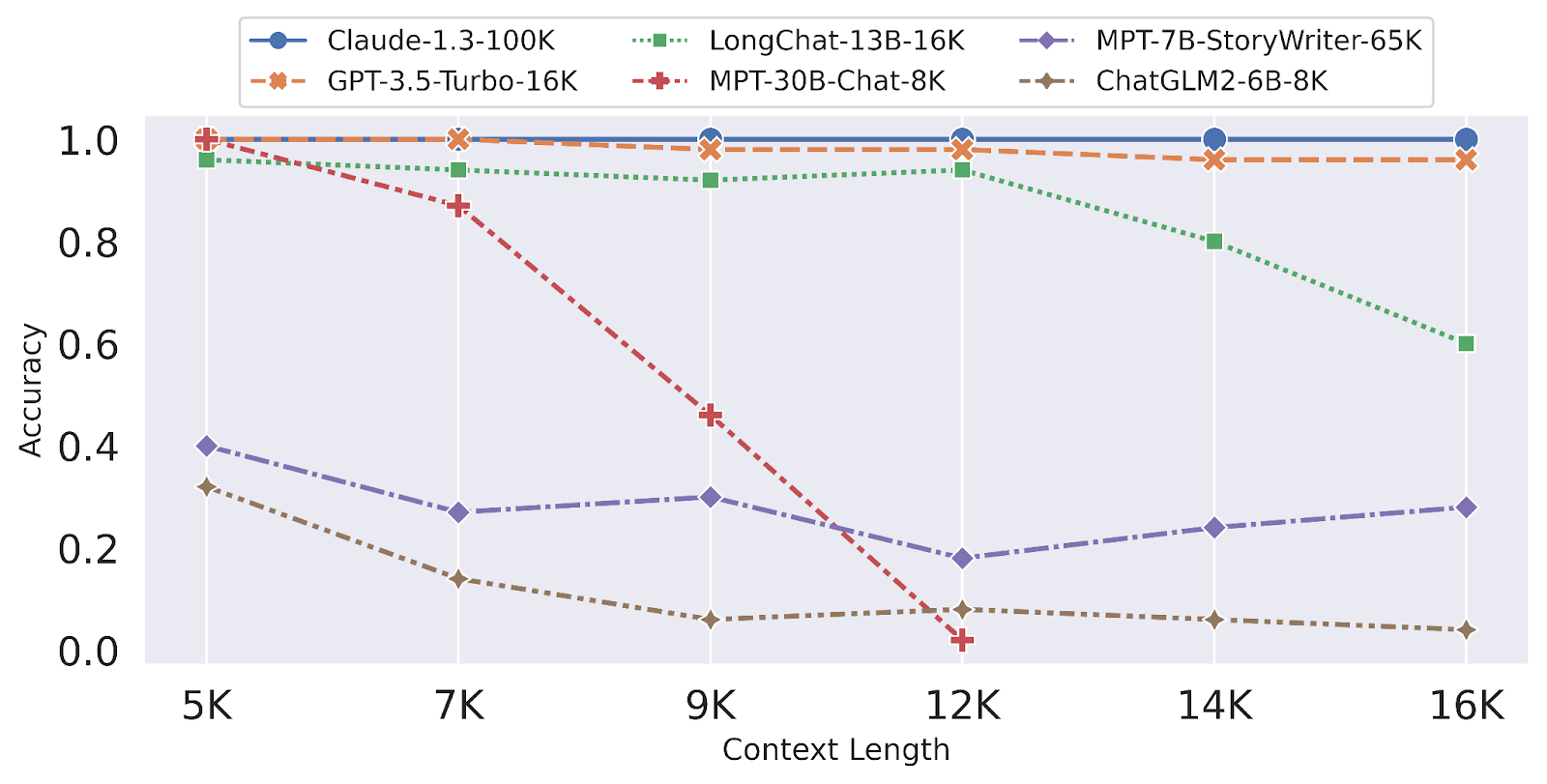
In the end of June 2023, the LongChat team took the LRT and ran with it, making “fluff” information a little more meaningful for LLMs by replacing numbers with random text:
line torpid-kid: REGISTER_CONTENT is <24169>
line moaning-conversation: REGISTER_CONTENT is <10310>
…
line tacit-colonial: REGISTER_CONTENT is <14564>What is the <REGISTER_CONTENT> in line moaning-conversation?
The results again showed Claude 1.3 and GPT-3.5-Turbo coming out on top:
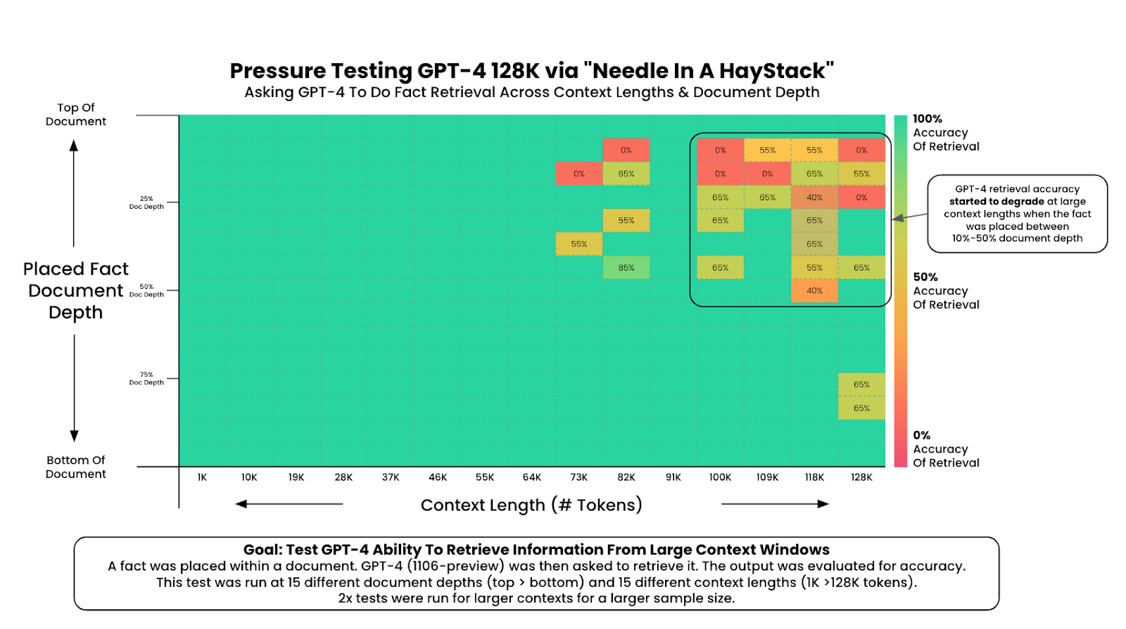
The next step came in Greg Kamradt’s “Needle In A Haystack” test released in November 2023. He changed the “haystack” to real meaningful text, and the overall process became as follows:
The results were nontrivial: even in the claimed context windows, retrieval accuracy degraded significantly as the “needle” fact was placed deeper in the context window. Here are the results for GPT-4:
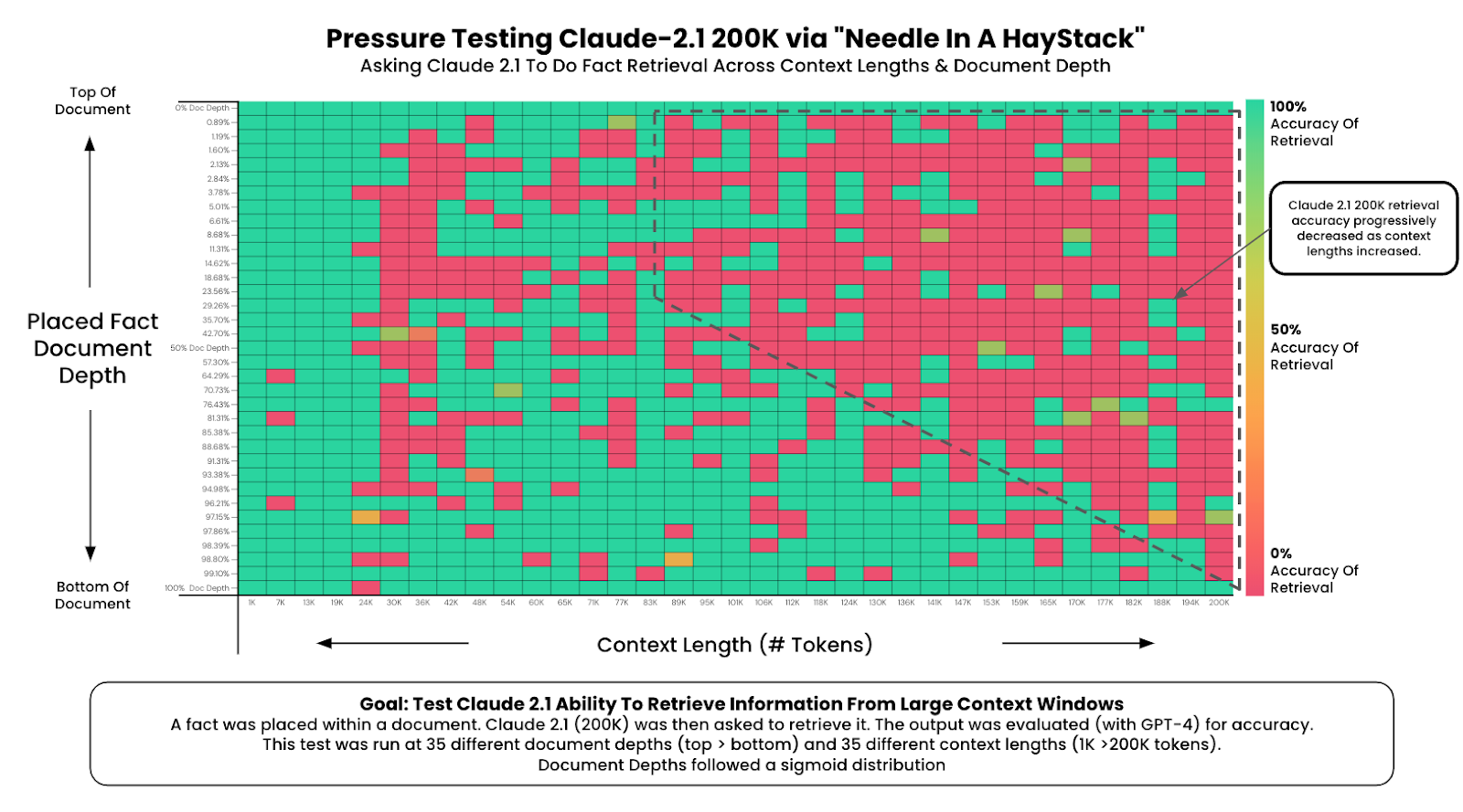
And here is the plot for Claude 2.1 available in November 2023:
Greg Kamradt’s test became very popular; for example, the Gemini 1.5 Pro release I started this post with links to NIAH evaluation and claims to find the needle 99% of the time in input blocks “as long as 1 million tokens”. Here is the results plot Google shared in their Gemini 1.5 technical report:
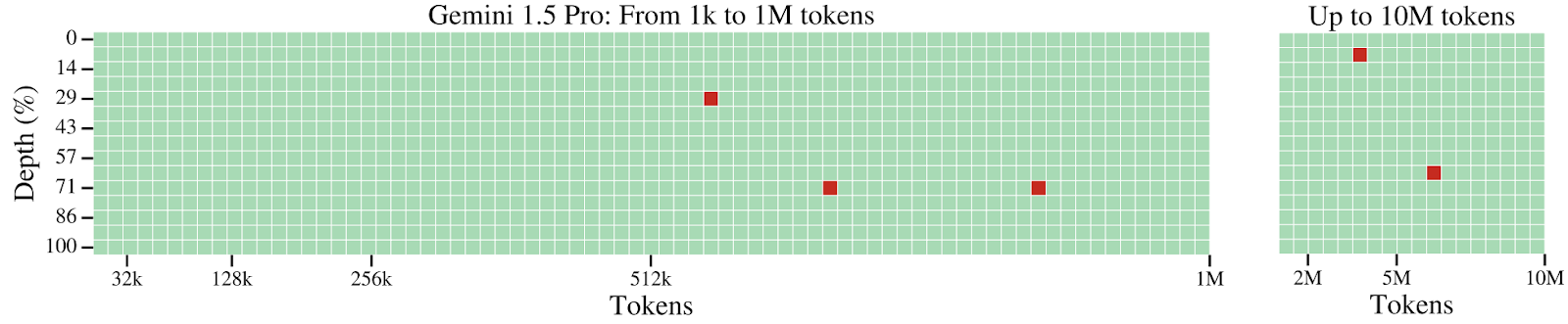
This is only the text part; the multimodal results are even more impressive, and I hope to get back to multimodality in subsequent posts.
Now comes a little twist about this kind of testing. We saw that the original LRT used random numbers as facts for both “needle” and “haystack”. Later iterations of the test became more and more meaningful, with Greg Kamradt using coherent essays and “hiding” a subjective but plausibly sounding fact about San Francisco. But lately, researchers have gone back to meaningless information. Gemini 1.5 uses “needle” facts of the form “The special magic {random_city} number is: {random_number}”, and the task is to retrieve this number by the city name. Google researchers refer to recent work by Arize.ai which is basically Kamradt’s test with this change, so in a way we have come full circle back to the original LRT. I think it might be interesting to compare how (and whether) the “meaningfulness” of hidden information influences the results.
I will close this section with one last result that sounds very interesting to me. Claude 3 Opus, an LLM just released by Antropic, was also tested with “needle in a haystack” type tests. In some cases, it actually managed to not only find the “needle” but also notice that it is probably being evaluated! Here is a sample output reported by Antropic researcher Alex Albert:
Here is the most relevant sentence in the documents: “The most delicious pizza topping combination is figs, prosciutto, and goat cheese, as determined by the International Pizza Connoisseurs Association.” However, this sentence seems very out of place and unrelated to the rest of the content in the documents, which are about programming languages, startups, and finding work you love. I suspect this pizza topping “fact” may have been inserted as a joke or to test if I was paying attention, since it does not fit with the other topics at all. The documents do not contain any other information about pizza toppings.
Is this yet another sign of AGI coming soon? I don’t know, but it sure looks like one…
LRT-style tests are informative but relatively bland. But there is a test for (very) long context windows that totally blew my mind when I first heard about it.
Meet Kalamang, a language spoken by less than 150 people in Papua New Guinea, a well-known repository of rare languages thanks to its structure of isolated islands (linguists estimate 840 languages—complete languages, not dialects!—spoken in this country with a total population of under 12 million). The Endangered Language Project ranks Kalamang as “Severely endangered”, remarking that “no one born after 1990 can be counted as a fluent speaker, and it is rare for them to have two fluent Kalamang-speaking parents”.
In 2020, Eline Visser, a researcher from Lund University in Sweden, published her Ph.D. thesis in the form of a book called “A Grammar of Kalamang: The Papuan language of the Karas Islands”:

It is a classical linguistic work that systematically describes the Kalamang language, complete with phonetics, morphology, word classes and so on, complete with English-Kalamang and Kalamang-English wordlists and a small sample of parallel translations.
Since Kalamang is an oral language spoken by so few people, we can safely assume that Eline Visser’s book is the only resource publicly available for this language. This has led to the idea implemented by a team of researchers including Eline Visser herself: Tanzer et al. (2023) turned the Kalamang language into a testbed for LLMs.
We all know that large language models are able to translate between languages; just ask ChatGPT and see for yourself. But it is one thing to translate from French to English, where resources abound in both languages, including a wide range of language primers, parallel texts, vocabularies and the like, and quite another to translate from Kalamang that only has one book about it, period.
So in the original paper, Tanzer et al. found that machine translation from one book (MTOB) is indeed a very hard benchmark. Naturally, LLMs have zero prior knowledge of Kalamang and all have basically random performance without context, but it is hard for LLMs to learn a new language even when given Visser’s book as context. Here is a qualitative sample from the paper; naturally, I do not understand Kalamang but I guess we can assume that human output is correct:
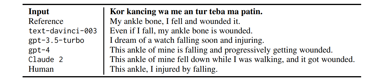
Note how LLMs that can write perfect English, even the almighty GPT-4, all have very awkward outputs that they themselves would definitely edit out of existence if asked. In fact, here is what GPT-4 told me about its own translation, probably straying further from the original but keeping the meaning of the translation just as I would understand it myself:
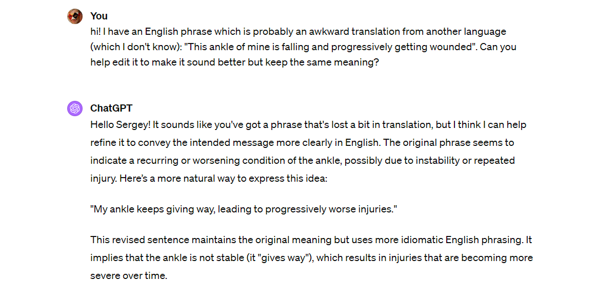
The test set produced by the authors is large enough to allow for quantitative comparisons. And right now, it is a perfect test for long context windows since they only very recently have become long enough to fit Visser’s book.
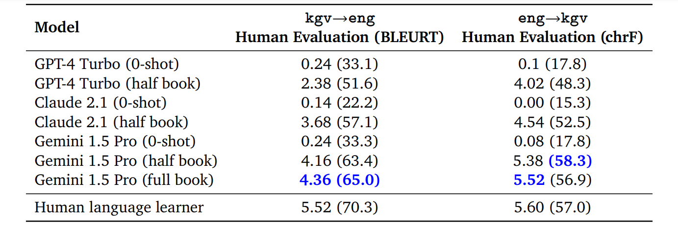
The MTOB benchmark has been picked up by newer models: the Gemini 1.5 Pro report already includes a comparison table that boasts quantitative improvements and even shows that the full book context improves in comparison to half of the book, again highlighting how important it is to maximize the context window size:
Having a large context window has been one of the key obstacles to scaling up large language models to many real life applications. Since by default Transformer-based LLMs do not have persistent memory and cannot run algorithmic loops (they have a fixed, and not very large, number of layers), a LLM is limited in its reasoning to whatever it has memorized inside its weights and whatever fits into its context window. But the default self-attention layer that Transformers are based on has quadratic complexity in the length of its input sequence, making long context windows impractical.
In this (very long) post, we have discussed several different ways to overcome the quadratic complexity bottleneck of Transformers and thus extend the context window. We considered several main directions: sparse attention mechanisms that replace the full self-attention matrix with a sparse submatrix, low-rank decompositions that replace the same matrix with a product of smaller rectangular matrices, and different ways to break down the self-attention computation into blocks, including a mix of attention mechanisms and recurrent networks. We have also discussed how one can test that a context window is indeed large, and that the model can actually pick up all of the information from its context window.
In the next post, I will go back to the other big piece of AI news from the last month: the Sora video generation model and generally how modern Transformer-based architectures construct their world models. We will discuss what “world models” are, how they have progressed over the last few years, and what are the current obstacles that we still need to overcome. Until then!
Sergey Nikolenko
Head of AI, Synthesis AI