AI Safety IV: Sparks of Misalignment
This is the last, fourth post in our series...
Here at Synthesis AI, we have decided to release the “Generative AI” series in an e-book form; expect a full-fledged pdf with all the images soon. But when I started collecting the posts into a single coherent whole, I couldn’t help but feel the huge, glaring omission of the most important topic in modern AI, the secret sauce that drives the entire field of ML nowadays: self-attention layers introduced in the original Transformer architecture. I haven’t planned to cover them before since there are plenty of other excellent sources, but in a larger format Transformers have become an inevitability. So today, I post the chapter on Transformers, which seems to be by far the longest post ever on this blog. We will discuss how the Transformer works, introduce the two main families of models based on self-attention, BERT and GPT, and discuss how Transformers can handle images as well.

The Transformer was introduced in 2017, in a paper by Google Brain researchers Vaswani et al. with a catchy title “Attention is All You Need”. By now, it is one of the most important papers in the history of not only machine learning but all of science, amassing nearly 100000 citations (by Google Scholar‘s count) over a mere five years that have passed since its publication.
An aside: for some unknown reason, it is quite hard to Google the most cited papers of all time, and there is no obvious way to find them on Google Scholar. I have found an authoritative review of the top papers of all time in Nature, and it cites only three papers with over 100K citations in the entire history of science, but those are “proper” citations counted by the Web of Science database. Lowly arXiv preprints do not register at all, so their numbers are always far lower than on Google Scholar that counts everything. In any case, the Transformer paper is truly exceptional.
There have been dozens of surveys already, so I will cite a few but it is far from an exhaustive list: (Zhou et al., 2023; Wolf et al., 2020; Lin et al., 2022; Tay et al., 2022; Xu et al., 2023; Wen et al., 2022; Selva et al., 2023). The Transformer was indeed a very special case, an architecture that, on one hand, uses ideas already well known in the machine learning community for many years, but on the other hand, combines them in a whole that has proven to be much, much larger than its parts. So what is the basic idea of a Transformer?
First, the original Transformer was an encoder-decoder architecture intended for sequence-to-sequence problems, specifically for machine translation. In essence, the original Transformer was designed to:
This means that before starting to encode text, the Transformer needs to convert it into a sequence of tokens; we will talk about it more in the next section, and for the images here let us just assume that tokens are individual words. After that, the original Transformer had the following structure:
Here is this structure:
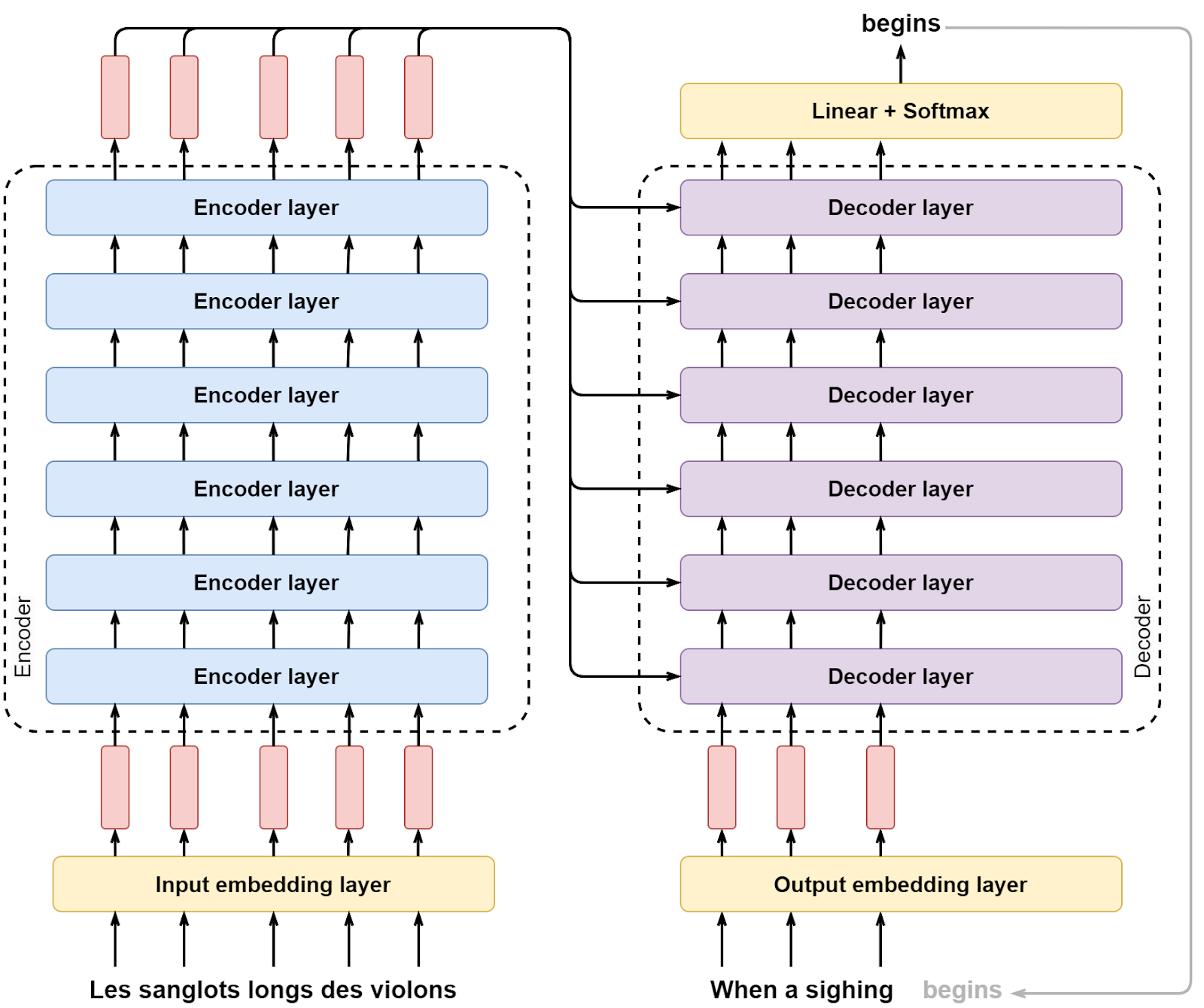
Each layer has a very simple internal structure:
Here is what the Transformer looks like with a single layer expanded in both encoder and decoder:
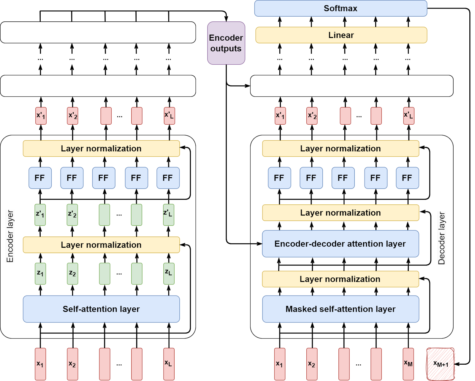
Layer normalization (Ba et al., 2016) is just a standard technique to stabilize training in deep neural networks; in the Transformer, it is also combined with a residual connection, so it is actually LayerNorm(X + Z), where X is the matrix of original input vectors x1,…,xL and Z is the matrix of the self-attention results z1,…,zL. A feedforward layer is just a single layer of weights applied to the vectors z’1,…,z’L.
The real magic happens in the self-attention layers, both in regular self-attention and encoder-decoder attention layers featured in the decoder. Let us look at them in more detail.
The intuition for self-attention layers comes from information retrieval, a field that we have already considered in detail in Part IV of this series. For the Transformer, we only need the very basic intuition of searching in the latent space, as illustrated below:
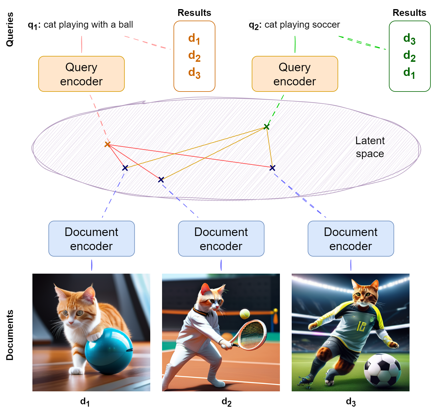
In this simple form, information retrieval works as follows:
In the self-attention layer, this intuition comes alive in a very abstract fashion. Let us follow through this process as it is illustrated below:
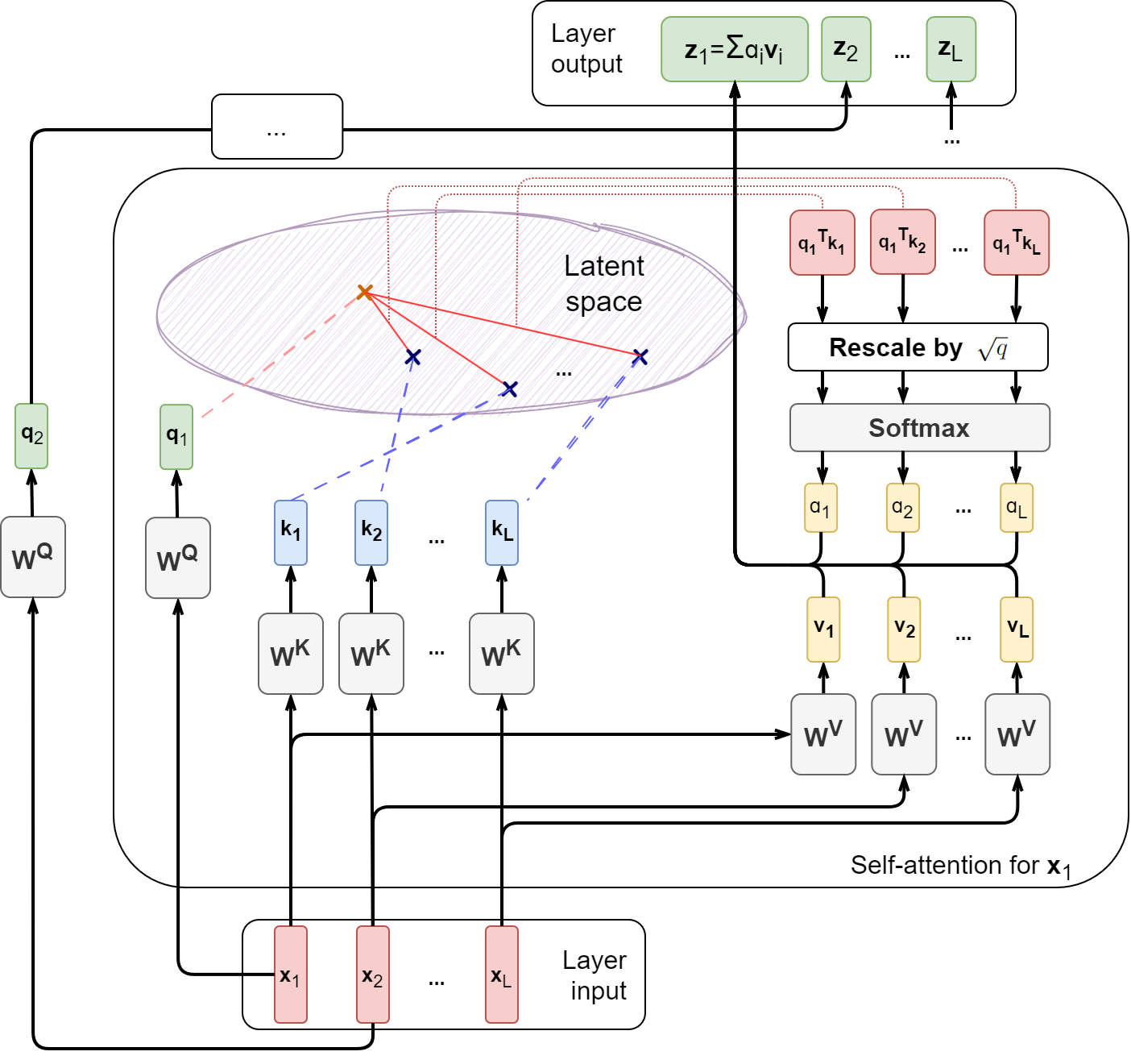
The self-attention layer receives as input a sequence of vectors x1,…,xL, which we can think of as a matrix X∊ℝd⨉L.
First, what are the queries, keys, and documents? All three of them come from the vectors xi themselves! The figure above shows this idea with the example of what happens with x1:
The matrices WQ, WK, and WV comprise the bulk of trainable weights in the self-attention mechanism. After applying them as above, we obtain three vectors {qi, ki, vi} from each input vector xi. Then we do the retrieval part, computing attention scores as scalar products between queries and documents. The figure above shows this process schematically with the example of q1 transforming into q1Tvi for all different i. Then we need to rescale q1Tvi, dividing it by the square root of q, and pass the scores through softmax to turn them into probabilities. The self-attention weights are thus

where K ∊ ℝq⨉L are all the keys combined in a matrix, K = WKX.
Then we use the result as coefficients for a convex combination of values vj. Thus, overall we have the following formula for what xi turns into:

where V ∊ ℝv⨉L are all the values combined in a matrix, V = WVX.
The normalizing factor comes from the fact that if you add q random numbers distributed around zero with variance 1, the result will have variance q, and the standard deviation will be the square root of q. So if you add 64 signed numbers that are around 1 in absolute value, the result will be around 8. It would be easy to saturate the softmax with this extra factor, so to get the numbers back to a reasonable range we divide back by the standard deviation.
We can combine the computation of each zi shown above into a single formula in matrix form, which is how self-attention is usually defined:

But this is only one way to “look at” the input vectors! What we have defined now is not the full self-attention layer but only a single self-attention head. We want to parallelize these computations along H different heads, using different weight matrices WQ1,…,WQH, WK1,…,WKH, and WV1,…,WVH to allow the Transformer layer to consider different combinations of the same input vectors at once. This process, known as multi-head attention, is illustrated below:
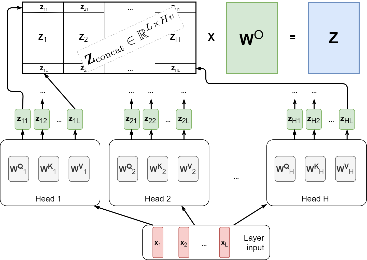
Note that after H parallel heads, we get H output matrices Z1,…,ZH, each of dimension v⨉L. We need to compress them all into a single output matrix Z ∊ ℝd⨉L with the same dimension as the input matrix X so that we can stack such layers further. The Transformer does it in the most straightforward way possible, as shown in the figure: let us just concatenate them all into a single large matrix Zconcat ∊ ℝL⨉Hv and then add another weight matrix WO ∊ ℝHv⨉d that will bring the result back to the necessary dimension:

With the output weight matrix WO, we allow the self-attention layer to mix up representations obtained from different attention heads; this is also an important way to add more flexibility and expressiveness to the architecture.
We are now entirely done with the self-attention layer but not quite done with the entire architecture. We have already discussed the rest of an encoder layer: after the multi-head attention, we use layer normalization with a residual connection LayerNorm(X + Z) and then add a feedforward layer that mixes features inside each of the token representations, with another residual connection around it leading to another LayerNorm, as shown inside the encoder layer in the general figure above.
This has been the most important part, but there are still quite a lot of bits and pieces of the Transformer architecture to pick up. In the next section, we will discuss how the decoder part works, how the input embeddings are constructed from text, and what the original Transformer architecture actually did.
We have discussed the main idea of self-attention and seen how it comes together in the encoder part of a Transformer. Let us now turn to the right part of the general figure shown above that has two more layer types that we do not know yet: masked self-attention and encoder-decoder attention. Fortunately, they are both now very easy to introduce.
Masked attention basically means that since the decoder works autoregressively, it should not peek at the tokens that it has not produced yet. This could be done by changing the input, but it’s easier and faster to just have the whole sequence and masking future positions inside self-attention layers themselves. Formally this means that in the self-attention formula, we set the softmax arguments to negative infinity for future tokens, which means that their attention weights will always be zero.
Encoder-decoder attention is a variation on the self-attention mechanism that takes into account the results of the encoder. These results are vectors with the same dimension as the output matrix Z that we obtained in the formula above, that is, L vectors of length d, and the figure suggests that each layer in the decoder receives these vectors as a condition.
It might seem to require a very different architecture to condition self-attention on this matrix… but in fact it’s an almost trivial modification. We have the exact same self-attention layer described above, with weight matrices that create queries, keys, and values for every attention head, but use different vectors as input:
Informally, this means that we are doing “retrieval” on the encoder’s output with queries made of already produced tokens. Formally, we simply use the same formula with queries, keys and values defined above, and all dimensions match nicely: there are L terms in the softmax argument for each vector, but the number of queries and hence number of outputs matches the number of inputs.
Note also that the decoder has an extra linear layer at the end followed by a softmax for next token classification; this is about the simplest classification head possible, obviously needed for the decoder.
But this is still not all. We need to discuss one more thing: how does the input text turn into a sequence of dense vectors that self-attention layers process so skillfully? There are two things to discuss here.
First, tokenization. I have mentioned above that tokens do not really correspond to words. In most Transformer-based models, tokenization is done with a process known as the byte-pair encoding, an interesting idea in its own right based on optimal coding theory such as, e.g., Huffman coding. To begin with, we consider all words present in the input text (the notion of a “word” should be understood liberally, but it is, more or less, a sequence of characters delimited by whitespace) and count the number of their occurrences, building a vocabulary. Let us consider a few words that share a lot of repeating character subsequences:
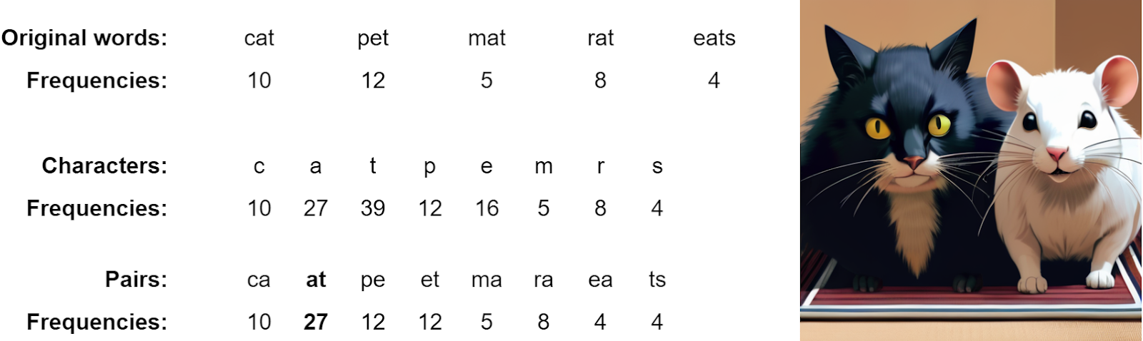
We first count the word frequencies, as shown above. Then we break down this vocabulary into individual symbols and count them; in practice there would be extra symbols for the beginning and/or end of a word and all sorts of extra stuff, but let’s keep it simple and stick to our “cat on a mat” example; this is the middle part of the figure above.
This is our original vocabulary of symbols, and now the encoding process can begin. We break down the symbols into pairs and count their occurrences:
{ ca: 10, at: 27, pe: 12, et: 12, ma: 5, ra: 8, ea: 4, ts: 4 }.
Then we choose the most frequent pair—in this case “at“—and re-encode it with a single new symbol that is added to the vocabulary; let’s call it Z. After that, we have a new set of words in the new encoding, and we can count the symbols and their pairs again:
{ cZ: 10, pet: 12, mZ: 5, rZ: 8, eZs: 4 },
{ c: 10, Z: 27, t: 12, p: 12, e: 16, m: 5, r: 8, s: 4 },
{ cZ: 10, pe: 12, et: 12, mZ: 5, rZ: 8, eZ: 4, Zs: 4 }.
At this point, we can choose the new most frequent pair—in this case “pe” or “et“—and replace it with another new symbol, say Y. Replacing “pe“, we get the following new vocabulary and statistics:
{ cZ: 10, Yt: 12, mZ: 5, rZ: 8, eZs: 4 },
{ c: 10, Z: 27, Y: 12, t: 12, e: 4, m: 5, r: 8, s: 4 },
{ cZ: 10, Yt: 12, mZ: 5, rZ: 8, eZ: 4, Zs: 4 }.
As we run the algorithm in a loop, new symbols may also become part of new pairs; in our example, the next most frequent pair is “Yt“, so after the next step we will have a whole separate token corresponding to “pet“. Note that we never remove symbols from the vocabulary even if they have zero occurrences after a merge: we may not have any t‘s left after the next merge, but new input text may contain new unknown words with t‘s that will need to be processed, so we need the vocabulary to stay universal.
The encoding process can be stopped at any time: on every step, we get a new extended set of tokens (vocabulary) that compresses the original text in a greedy way, and we can stop and use the current set of tokens. So in practice, we set a target vocabulary size and run the algorithm until the set of tokens reaches this size, usually getting excellent compression for the original text in terms of these new tokens. As a result, words may still be broken into parts, but the most frequent words will get their own tokens, and the parts themselves may have meaning; for example, in English it would be expected to have a token like “tion” appear quite early in the process, which is a frequent sequence of letters with a clear semantics.
That’s it for tokenization! At this point, the input is a sequence of fixed discrete objects (tokens) taken from a predefined vocabulary of size V. It remains to turn it into a sequence of dense vectors x ∊ ℝd, which is usually done via an embedding layer that’s just basically a large d⨉V matrix that consists of trainable weights. In earlier days of the deep learning revolution in natural language processing, word embeddings were a quite interesting field of study in and of themselves because they used to be trained separately and then just applied as a fixed “dense vocabulary” that neural models trained on top of. This field of study has given us word2vec (Mikolov et al., 2013a; 2013b; Le, Mikolov, 2014), GloVe (Pennington et al., 2014), and many more interesting ideas… but there is no point to discuss them here because now it’s just a trainable layer like any other, and the whole architecture is being trained at once, including the embedding layer.
Still, there is another point about the embeddings which is unique to Transformers. One of the main characteristic features of the Transformer architecture is that every input token can “look at” any other input token directly, with no regard for the distance between them in the input sequence. The self-attention layer has a separate attention weight for every pair of tokens, not just neighboring ones or something like that. This has a drawback too: the length of the input, which for language models is known as the context window, automatically becomes bounded. But this is a big advantage over, say, recurrent architectures where you need to go through every step of the sequence, “losing memory” along the way, before the influence of one word can reach another.
But there is another interesting consequence of this property: since the attention weights cover all tokens uniformly, we lose the sequence. That is, for a self-attention layer there is no sense of some tokens being “next to each other” or “closer in the input sequence”, it is all just a single matrix of weights. We need to give the Transformer an idea of the input sequence artificially; this is done via the so-called positional encodings.
Positional encodings are vectors added to the embedding that reflect where in the sequence the current token is; we will discuss them briefly but I also refer to a more detailed description of positional encodings by Kazemnejad (2019). How could we encode the position? Well, we could have a number that is increasing with the position but it is hard to get right:
Therefore, the Transformer uses a very clever idea inspired by how we encode numbers in our regular positional notation. Consider a sequence of numbers, say written in binary, like on the left of the figure below:
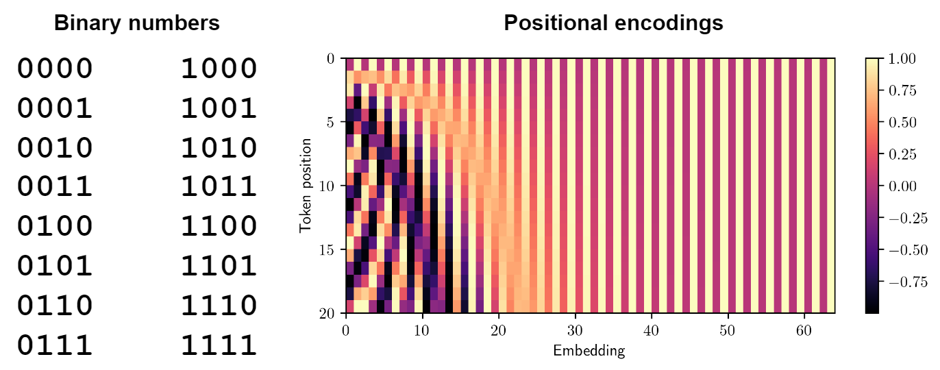
As the numbers increase, the value of each digit forms a periodic function, with different periods for different digits in the number. We want to replicate something like that in the positional encodings, but since we have the full power of real numbers available now, we use continuous periodic functions, sine waves:

where pos is the token position in the sequence and d is the embedding dimension. This means that each cell in the has a sine wave with respect to the position (half of them shifted to a cosine wave), each with its own period that is increasing with i, that is, with the cell index. The result is shown in the figure above on the right, where the horizontal axis shows the cell indices i and the vertical axis shows token positions from top to bottom. Sine waves become more and more elongated (with increasing period) as we go from left to right, so for 20 tokens we are actually using only about 20-25 dimensions for the positional encoding, but this definition can support arbitrarily long input sequences, even longer than those present in the training set.
It was a little surprising to me that positional encodings are not concatenated with regular embeddings but rather added to them. It looks counterintuitive because positional information is different and should not be mixed with token semantics. But embeddings are learned rather than fixed, and as you can see in the figure, positional encodings take up a small portion of the overall vector, so they can probably coexist just fine. In any case, the input embedding is a sum of the trainable embedding for the current token and the vector PE(pos, i) defined above.
And with that we are completely done with the Transformer architecture, so let us briefly discuss its original results. As I have already mentioned, the original Transformer presented by Vaswani et al. (2017) was doing machine translation, and numerically speaking, results of the original Transformer architecture were not the most striking: the encoder-decoder architecture applied to machine translation scored roughly on par with the best existing models in English-French and English-Deutsch translations. But the Transformer had equally good BLEU scores in machine translation… while requiring 100x less compute for training! And when you have an architecture with 100x less compute, in practice it means that you can train a much larger model (maybe not exactly 100x larger, but still) with the same computational budget, and then you will hopefully scale to much better results.
Since 2017, Transformers have become one of the most popular architectures in machine learning. In the rest of this post, we will discuss some further extensions and modifications that the Transformer has undergone, although surprisingly few have been necessary to adapt the architecture even to entirely new data modalities.
As we have discussed in the previous section, the basic Transformer is a full-scale encoder-decoder architecture, where the encoder produces semantically rich latent representations of text in the input language, and the decoder turns them into text in the target language by writing it autoregressively.
From there, it was only natural to cut the Transformer in two:
Let us begin with the latter, i.e., with the decoder, but first let us understand in slightly more detail what we are talking about.
A language model is a machine learning model that predicts the next token in a sequence of language tokens; it is easier to think of tokens as words, although in reality models usually break words down into smaller chunks. The machine learning problem here is basically classification: what is the next token going to be? A language model is just a classification model, and by continuously predicting the next token, a language model can write text. We have already discussed it in Part VII of the series:
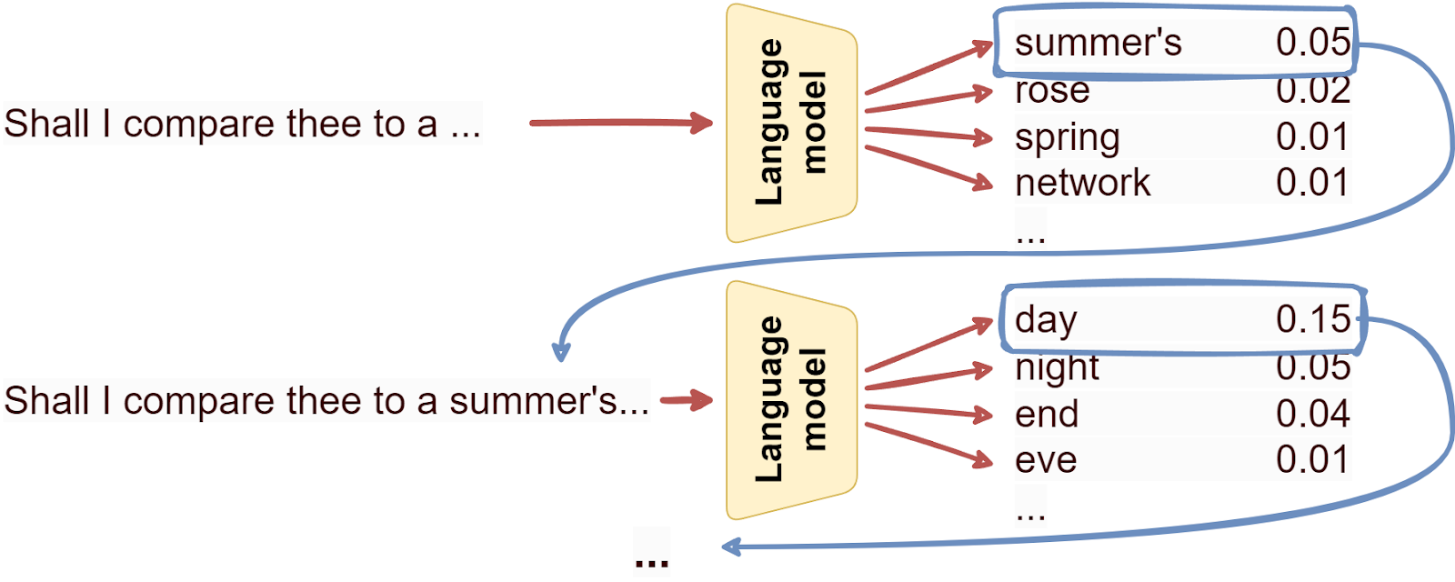
The only thing a language model can do: predict the next token, over and over. Note that this also means that there are very few problems with data collection or labeling for general-purpose language models: any human-written text becomes a set of labeled examples for supervised learning because the language model just predicts the next word, which is already there in the text. Therefore, you can just collect a lot of text off the Web and train on it! There are several standard datasets that are used to train large language models (LLMs) nowadays:
And now that we have these huge datasets, the language modeling part appears to be trivial: let us just use the Transformer decoder to autoregressively predict the next token! This exact idea was implemented in a series of models called Generative Pre-Trained Transformers — yes, that’s the famous GPT family.
In particular:
As the GPT family scaled up, it also obtained more impressive generalization abilities with regard to problems you might want to solve with it. Suppose, for example, that you wanted to recognize entailment relations, that is, find out whether a hypothesis sentence follows from a premise sentence. Data for this problem, e.g., the popular MultiNLI (Multi-Genre Natural Language Inference) corpus (Williams et al., 2018) looks like pairs of sentences labeled with three kinds of results:
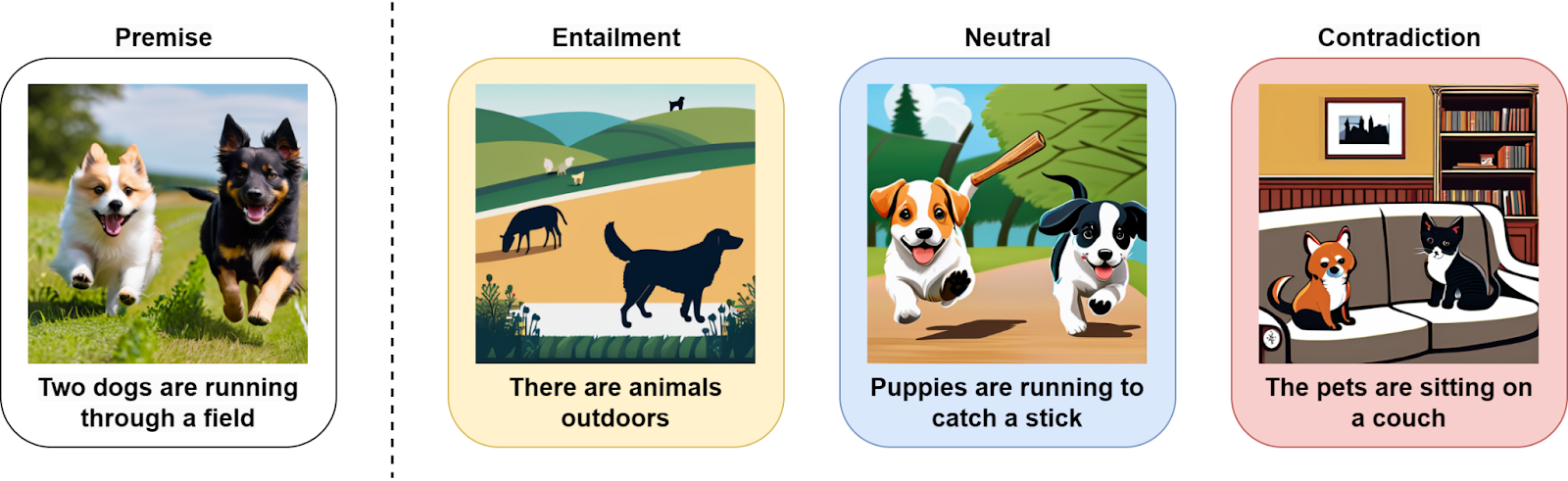
In the example above, for a premise “Two dogs are running through a field” (I took this example from Gugurangan et al., 2018),
Different versions of GPT and BERT would handle the entailment problem differently. To adapt the original GPT (Radford et al., 2018) or BERT (Devlin et al., 2018) to a specific task, you had to fine-tune it, i.e., modify its weights by performing additional training on the downstream task; you had to fine-tune the GPT model with a separate entailment dataset by encoding the dataset into a special form and training new weights for a separator embedding and a new linear layer on top. The figure below shows how this would work for the original GPT and details what new weights have to be learned. This is the way such problems had been processed in deep learning before, e.g., with large-scale recurrent architectures (Rocktäschel et al., 2015).
Starting from GPT-2, and definitely in GPT-3, developers of Transformer-based architectures moved to a different approach, where no new weights need to be trained at all. Similar to multitask learning and following an earlier attempt by the MQAN (Multitask Question Answering Network) model (McCann et al., 2018), they noted that a variety of different tasks could be encoded into text. Actually, one could argue that the Turing test is so good exactly because you can sneak in a lot of different questions into text-only conversations, including questions about the surroundings, the world in general, and so on. So to make use of a language model’s “understanding” (in this post, I’m putting “understanding” in quotes, but have you seen Part VIII?) of the world, you could give it a few examples of what you need and frame the problem as continuing the text in the prompt. The following figure compares the two approaches (GPT on the left, GPT-2 and 3 on the right) and shows a sample prompt for the logical entailment problem on the right; you would probably obtain better results if you put more examples in the omitted part of the prompt:
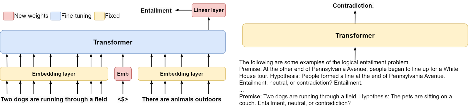
Note that in this approach, all that the language model is doing is still predicting the next token in the text, nothing more! Moreover, it is not even trained to do new problems such as entailment or question answering, it already “understands” what’s needed from its vast training set, and a short prompt with a couple of examples is enough to summon this “understanding” and let the model solve complex semantic problems.
A different way to cut up the original Transformer was introduced in the BERT model developed by Google researchers Devlin et al. (2018) . BERT stands for Bidirectional Encoder Representations from Transformers. As the name suggests, the main emphasis here is on learning semantically rich representations for tokens that could be further used in subsequent models, somewhat like word embeddings such as word2vec and GloVe had been used before but better and with full context available to the model producing representations.
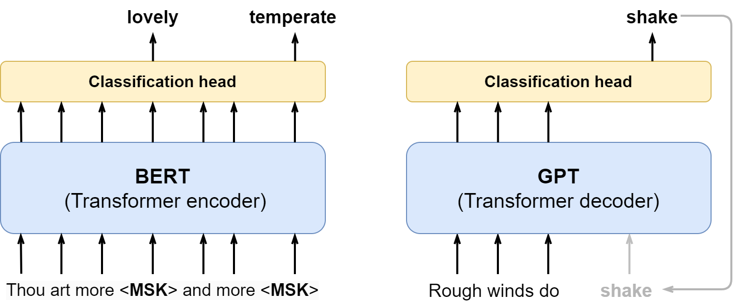
To do that, BERT leaves only the encoder part of the Transformer, the part that produces a semantically rich representation for each of the input tokens. But how do we train it if not with the language modeling objective that GPT uses? It turns out that we still can do approximately the same thing: instead of predicting the next token, we can mask out some of the tokens in the input (in the same way as we mask future tokens in the decoder) and predict them based on the full context from both left and right. This is known as masked language modeling, and it is the main pretraining objective for BERT.
Here is a comparison of the BERT (left) and GPT (right) pretraining objectives:
Just like language modeling itself, masked language modeling has a long history; it was originally known as the cloze procedure, introduced in 1953 as a readability test for texts in a natural language (Taylor, 1953). The word “cloze” is not a last name, it was derived from “closure”, as in gestalt psychology: humans tend to fill in missing pieces. So if you want to compare how “readable” two texts are, you delete some pieces from them at random and ask people to fill in the blanks: the most readable passage will be the one where the most humans get the most missing pieces right.
The original BERT combines two variations of this idea:
In later research, more models have been developed based on the Transformer encoder that can provide different flavors of embeddings with somewhat different properties. We will not do a proper survey here, referring to, e.g., (Zhou et al., 2023; Wolf et al., 2020; Lin et al., 2022), but let us mention a few of the most important BERT variations that have been important for natural language processing applications:
BERT and its derivative models such as RoBERTa have proven to be a very valuable tool for natural language processing (Patwardhan et al., 2023). The usual way to apply BERT has been to take the vectors it produces (BERT embeddings, or RoBERTa embeddings, or ALBERT, or any other) and plug them into standard neural models for various natural language processing tasks. This has usually improved things across the board, in problems such as:
Finally, another line of models that has been instrumental in modern NLP is XLM (cross-lingual language model; Conneau, Lample, 2019), a series of models based on BERT and GPT that trains on several languages at once. To do that, they apply byte-pair encoding to all language at the same time, getting a shared multilingual vocabulary, and use the same kind of LM and masked LM objectives to train in multiple languages at once. XLM and its successor models such as XLM-RoBERTa (Conneau et al., 2019) defined state of the art in many cross-lingual tasks such as the ones from XNLI, a cross-lingual benchmark for natural language inference (Conneau et al., 2018).
This has already turned into a high-level survey, so I think it is time to cut the survey short and just say that Transformers permeate absolutely all subfields and tasks of natural language processing, defining state of the art in all of them. But, as we will see in the next section, it’s not just natural language processing…
The Transformer immediately proved itself to be an excellent model for processing sequences of tokens. We will not speak of it in detail but sequences of other nature have also yielded to the magic of Transformers; for example, HuBERT soon became a standard model for speech processing (Hsu et al., 2021).
But images seem to be a different beast, right? An image has a natural two-dimensional structure, and deep learning has long had just the recipe for images: convolutional neural networks process every small window in the same way, sharing the weights in a form of ultimate structural regularization. Neural networks have been instrumental in the deep learning revolution, starting from AlexNet that made CNNs great again in 2011-2012 (Krizhevsky et al., 2012) and all the way to the automatically optimized architectures of the EfficientNet family (Tan, Le, 2019).
Well, it turns out that Transformers can help with images too! To do that, you need to convert an image into a sequence, and usually it is done in a very straightforward way. One of the first models that attempted it was Visual BERT (Li et al., 2019; Li et al., 2020), a model initially designed and pretrained for image captioning:
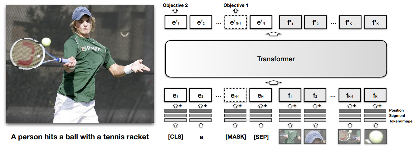
Since captions deal with objects that appear on an image, Visual BERT preprocessed the image with a fixed pretrained object detection system such as Faster R-CNN (Ren et al., 2015). Then the objects are cut out of the image, embedded into vectors via convolutional networks and special positional embeddings that indicate where the object was in the image, and just fed into a single Transformer:
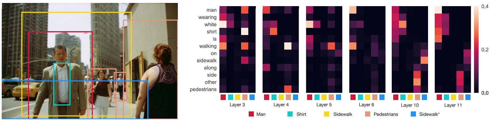
The figure above also shows sample attention heads and how words from the caption actually do attend to the objects that they describe or are closely related to.
The pretraining process closely follows how the original BERT is trained. Visual BERT has two pretraining objectives: masked language modeling where the task is to fill in the blanks in the caption and sentence-image prediction where the model needs to distinguish whether a given caption matches the image or not.
Similar ideas have been developed in many different BERT-based variations. Let me just note one of them: VideoBERT (Sun et al., 2019) that applied similar ideas to video captioning and processing, including text-to-video generation and forecasting future frames in a video:
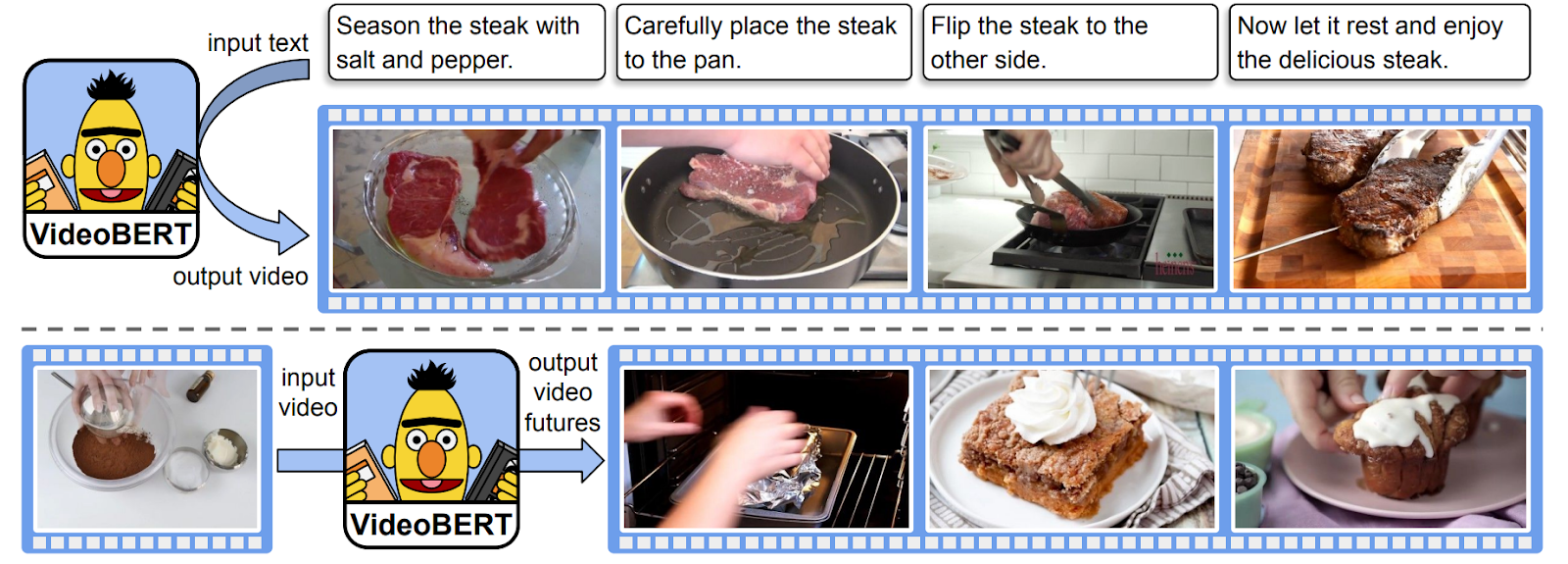
The figure above shows these problems: VideoBERT is able to predict the features of video frames corresponding to a given text (in this case a recipe), although it is, of course, better in the video-to-text direction, exceeding contemporary state of the art in video captioning.
VideoBERT is again pretrained with masked language modeling on a sequence of both text captions and video tokens:
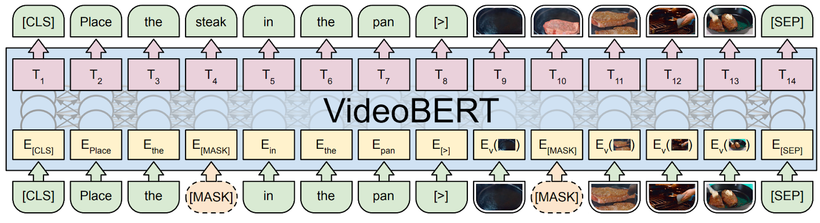
In this case, video tokens are obtained by sampling frames from the video, extracting features with a pretrained CNN, and tokenizing the features with simple k-means clustering. Both Visual BERT and VideoBERT were validated by experimental studies where they exceeded state of the art in visual question answering, image and video captioning, and other similar tasks.
But the most successful Transformer-based architecture for images has proved to be the Vision Transformer (ViT) developed in 2020 by Google researchers Dosovitsky et al. and introduced in a paper with a pithy title “An Image is Worth 16×16 Words“. Its original illustration from the paper is shown below:
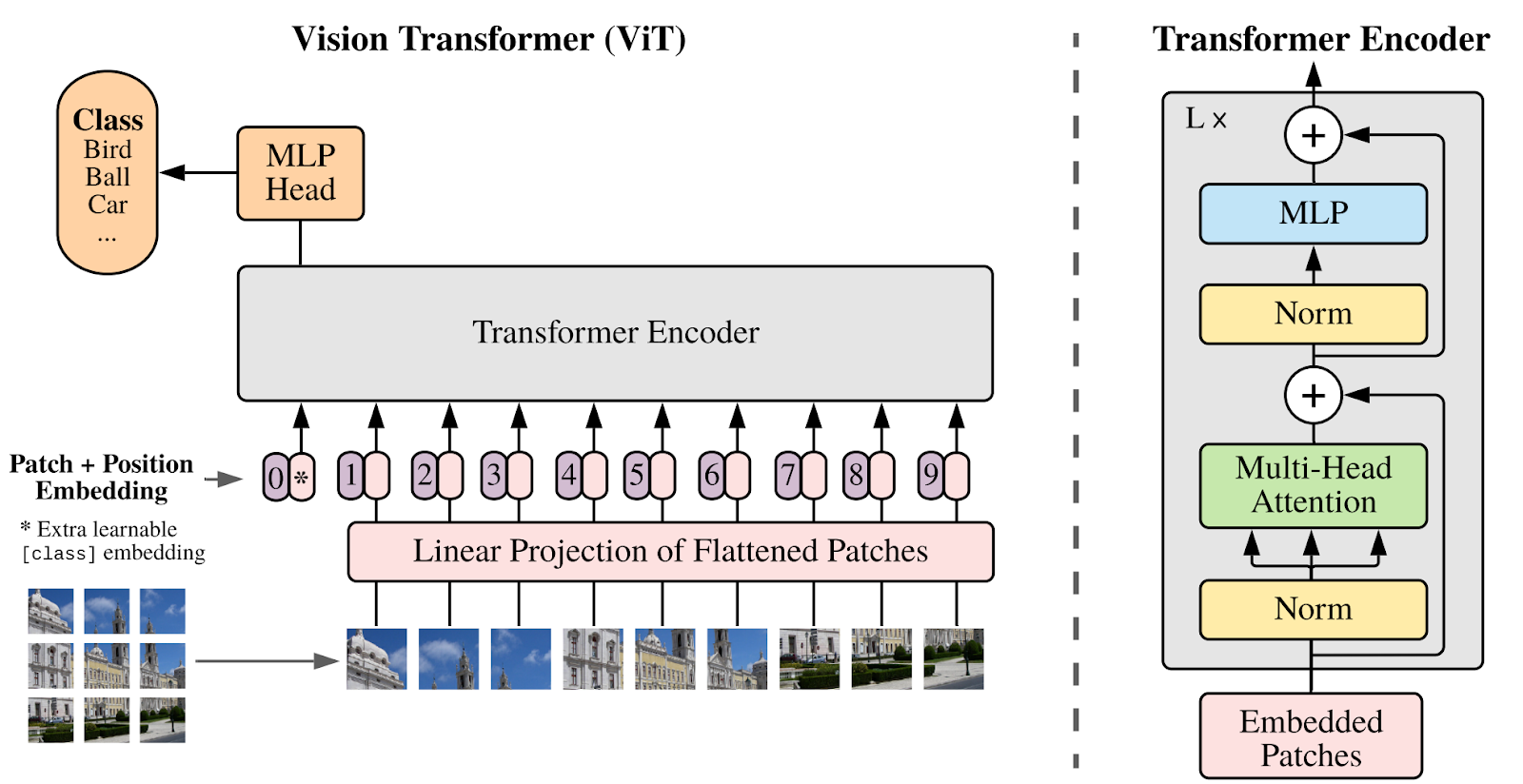
ViT is again basically a very straighforward modification of BERT. The difference is that now the model does not use text at its input at all, restricting itself to image-based tokens.
The input image into small patches: an H⨉W image with C channels xp ∊ ℝH⨉W⨉C becomes a sequence of patches xp ∊ ℝN⨉P·P·C, where N = HW/P2 is the number of P⨉P patches that fit into the original image (see the illustration above). The patches are turned into embeddings via a simple linear projection, and then the resulting sequence is fed into a Transformer encoder just like BERT. For pretraining, ViT uses masked patch modeling just like BERT does, replacing half of the input embeddings with the same learnable [mask] embedding and aiming to reconstruct the mean colors of the original patches.
Similar to the original Transformer, ViT uses positional encodings to add information about the sequence. What is even more striking, it is the same positional encoding as in the regular Transformer even though the geometry is now two-dimensional. Dosovitsky et al. report their experiments with positional encodings that would reflect the two-dimensional structure, but, surprisingly, this did not make any significant difference: one-dimensional positional encodings that we discussed above worked just as well.
Since 2020, ViT has been used for numerous different applications (we refer to the surveys by Guo et al, 2021 and Khan et al., 2022) and has had several important extensions that we will not discuss in detail but have to mention:
Finally, another important architecture that has added important new ideas to the Transformer is DeepMind‘s Perceiver (Jaegle et al., 2021a). It is a general-purpose architecture that can process numerous different modalities: images, point clouds, audio, and video, basically of any input dimension. The problem that the Perceiver has to solve is the quadratic bottleneck of Transformer’s self-attention: the formulas we showed above for the original Transformer have quadratic complexity in the input size. Importantly, it’s quadratic in a very specific part of the input size: you can project the queries, keys, and values into smaller dimensions but there is no escape from having quadratic complexity in the number of queries, i.e., the context window size.
The Perceiver avoids this bottleneck by using lower-dimensional latent units: it’s quadratic in the number of queries, so we use a small vector of latents for queries and can use large byte arrays as inputs for K and V, projecting them down to a lower-dimensional representation in cross-attention layers, as shown in the original illustration from Jaegle et al., (2021a):
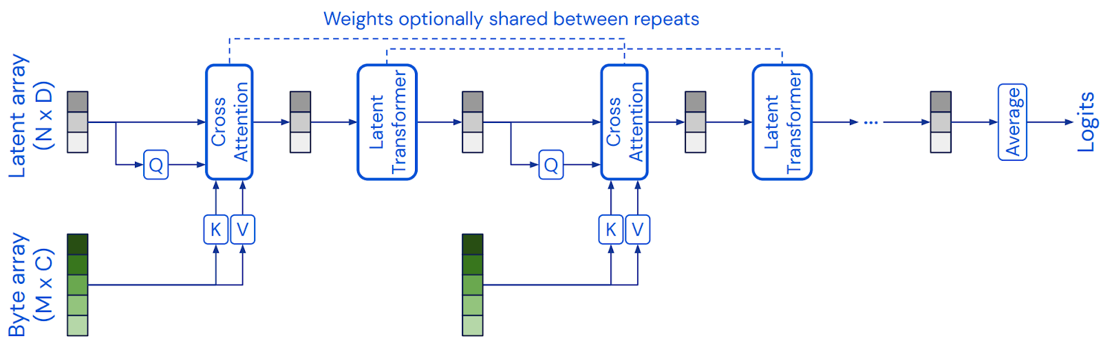
The cross-attention layer is the same as in the Transformer decoder (see above).
The next version of Perceiver, called Perceiver IO (Jaegle et al., 2021b), extended this idea to outputs as well as inputs. While the original Perceiver could only solve problems with low output dimensions, such as classification, Perceiver IO can also handle large output arrays such as high-definition images. It is done with a trick reminiscent of how NeRFs represent high-dimensional outputs with implicit functions (Mildenhall et al., 2020; Tancik et al., 2023): Perceiver IO uses a smaller output query array to process with cross-attention and then constructs the actual output queries for the large-scale final output in an automated way, by combining a set of vectors that describe properties of the current output such as position coordinates. The general structure looks like this:
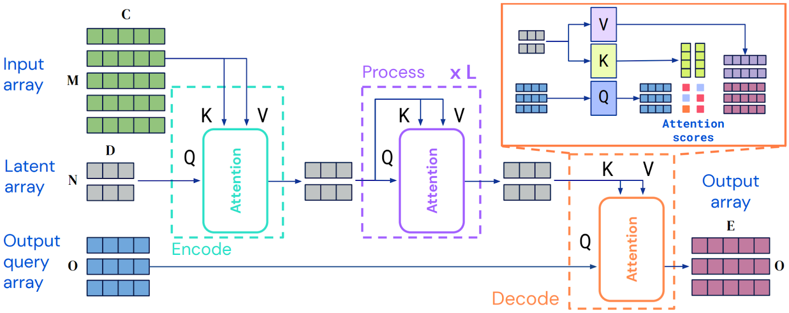
We will not go into more detail on this idea, but as a result Perceiver IO can handle high-dimensional outputs such as images or audio, which means it can scale to problems such as image segmentation, optical flow estimation, audio-video compression by autoencoding and so on.
In this series, we have used Vision Transformers in Part IV, where they served as the basic image encoders for the CLIP and BLIP models that will provide us with high-quality multimodal latent spaces for both multimodal retrieval and text-to-image conditional generation.
The idea of a self-attention layer, originally appearing in the Transformer encoder-decoder architecture in 2017, can be easily called the single most important idea in the last ten years of machine learning. Transformers have, pardon the obvious pun, transformed machine learning, getting state of the art results for all types of unstructured input data, including those that do not have an obvious sequential structure, like images that we have considered above.
Moreover, as we have seen in Part VII of this series, Transformers are becoming instrumental not only for the academic discipline of machine learning but also for the world economy. Transformative AI (TAI) that we have mentioned in Part VIII is named after an economic transformation similar to the Industrial Revolution, but it might prove to be yet another pun on the world’s most popular architecture.
Over the course of this “Generative AI” series, we have already taken Transformers and applied them in many different ways: generated discrete latent codes for VQ-VAE-based image generation models in Part III, mapped images and text into a common latent space in Part IV, encoded text to use it to condition diffusion-based models in Part VI, and upscaled straightforward language models from the GPT family into universal tools that find uses across many different industries in Part VII. Who knows, maybe Transformers will get us all the way to AGI, as we have discussed in Part VIII. In any case, it is hard to imagine modern machine learning without Transformers.
Sergey Nikolenko
Head of AI, Synthesis AI