AI Safety IV: Sparks of Misalignment
This is the last, fourth post in our series...
It might seem like generative models are going through new phases every couple of years: we heard about Transformers, then flow-based models were all the rage, then diffusion-based models… But in fact, new ideas build on top of older ones. Following our overview post, today we start an in-depth dive into generative AI. We consider the variational autoencoder (VAE), an idea introduced in 2013, if not earlier, but still very relevant and still underlying state of the art generative models such as Stable Diffusion. We will not consider all the gory mathematical details but I hope to explain the necessary intuition.

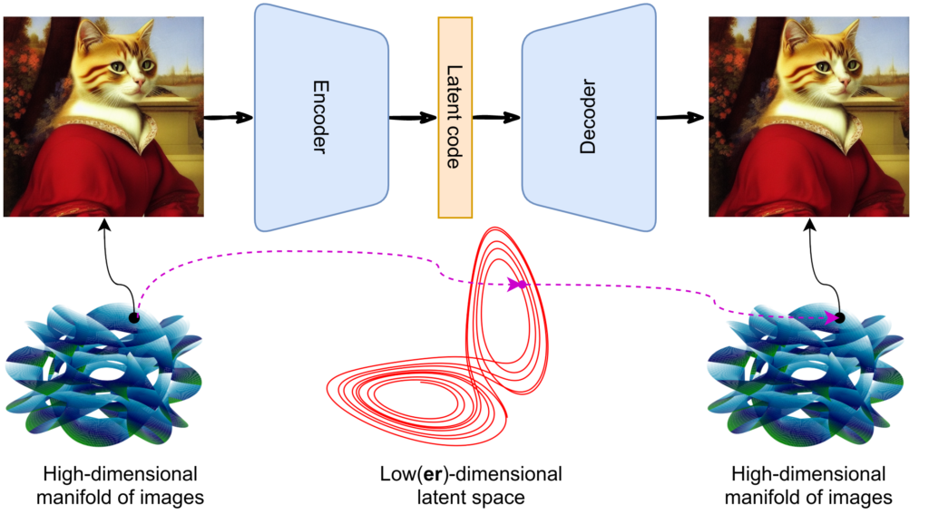
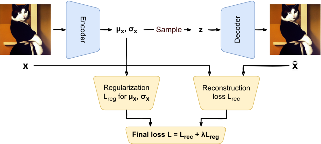
We already covered this basic idea in the overview post but let me reintroduce the problem and move on to a more detailed discussion of the VAE intuition. We discussed that a basic autoencoder can learn to compress and decompress images pretty well with a simple high-level architecture like this:

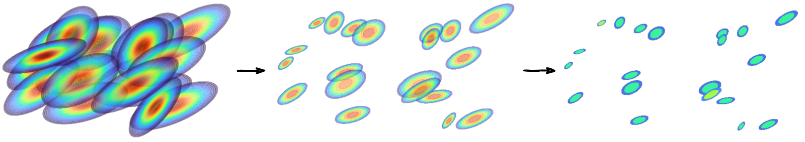
However, this is not enough to get you a generative model because the structure of latent codes will still be too complicated. You have a very complex manifold of images in a huuuuuge space with dimensions in the millions, but the latent space probably also has dimension in the hundreds or low thousands, and the latent codes will have a complicated structure in that space:
So if you try to sample latent codes from a simple distribution you will almost certainly fail, that is, your samples will fall outside the manifold of latent codes, and the decoder will fail to produce anything meaningful, let alone beautiful:

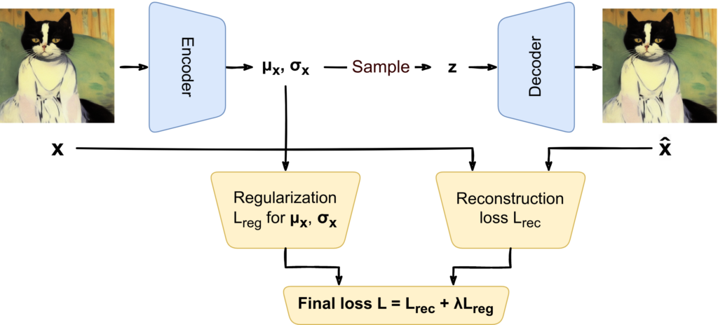
A variational autoencoder tries to fix this problem by making each point “wider”. Instead of a single latent vector z, now each input x is mapped to a whole distribution:
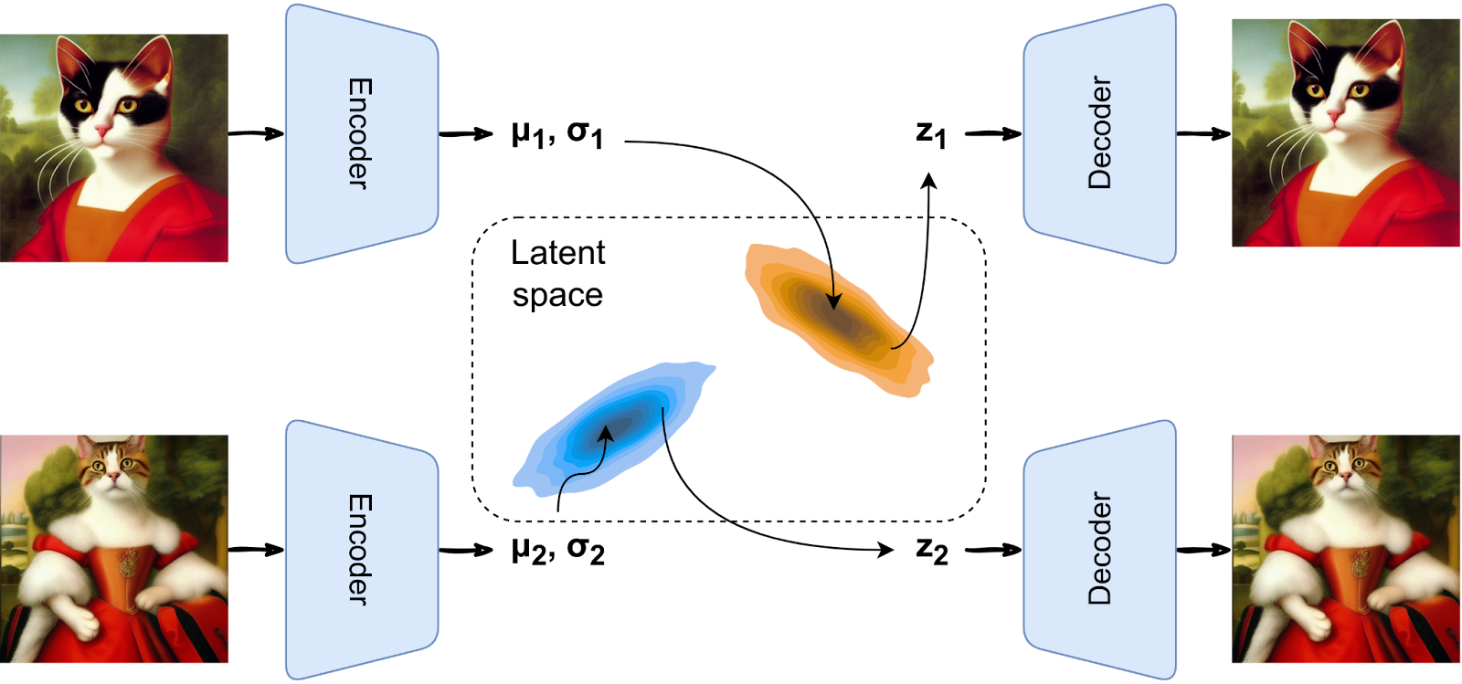
The intuition is that by making the decoder to work with z’s sampled from whole distributions, we force it to be robust to small changes in z. Ultimately, we want to cover a whole chunk of the latent space with points that have “reasonable” decodings, so that afterwards we can sample from a simple distribution and still get good results:
This idea, however, meets with two difficulties. First, when we begin to train an autoencoder, it will be beneficial for it to make the intermediate distributions as “small” (with low variance) as possible: if you are always very close to the central point the decoder’s job becomes easier, and reconstructions probably improve. In a similar vein, the distributions may begin to drift off from each other in the latent space, again making the decoder’s job easier as it now has more slack in distinguishing between different inputs. So unless we do something about it, the training process will look something like this, tending to a regular autoencoder that we know to be of little value for us:
To alleviate this problem, we need to impose some kind of a constraint on what’s happening with the intermediate distributions. In machine learning, hard constraints rarely appear, they usually take the form of regularizers, i.e., additions to the loss function that express what we want. In this case, we want to keep the distributions for each input x relatively “large” and we want to keep them together in relatively close proximity, so we probably will kill two birds with one stone if we make the distribution px(z | μx, σx) closer to a standard Gaussian. Our overall loss function now becomes a sum of the reconstruction loss and this regularizer:
Still, the question remains: how do we regularize? We want px(z | μx, σx) to be close to a standard Gaussian distribution, but there are several plausible ways to do that: the Kullback-Leibler divergence can cut both ways, either KL(p||q) or KL(q||p), and then there are combinations like the Jensen-Shannon divergence… What would be the best and conceptually correct way to define Lreg?
The second problem is more technical: the picture above has the latent code z sampled from a distribution px(z | μx, σx). This is fine during inference, when we want to apply the already trained encoder and decoder. But how do we train? Gradients cannot go through a “sampling layer”.
Let us begin with the first problem; solving it will also give us a nice probabilistic interpretation of what’s going on in VAE and explain why it is called a variational autoencoder.
Let us consider a different way to look at the same structure that leads to different insights and ultimately will help us understand the mathematical ideas behind variational autoencoders. We will start from scratch: suppose that we want to train an encoder to produce latent codes z from images x and a decoder to go back from z to x.
We begin with a very simple formula; I promised as little math as possible but, to be honest, there will be a little more than that below:

This is basically the Bayes formula in its simplest form: it says that the joint distribution of images and their latent codes can be decomposed in two different ways, starting either with p(x) or with p(z) and multiplying it by the corresponding conditional distribution.
We already understand, at least generally, all parts of this formula: p(x) is the distribution of images, p(z) is the distribution of latent codes, i.e., the simple distribution we want to be able to sample from (most likely a standard Gaussian), and the other two distributions are what we need to find, the encoder distribution p(z|x) and the decoder distribution p(x|z):
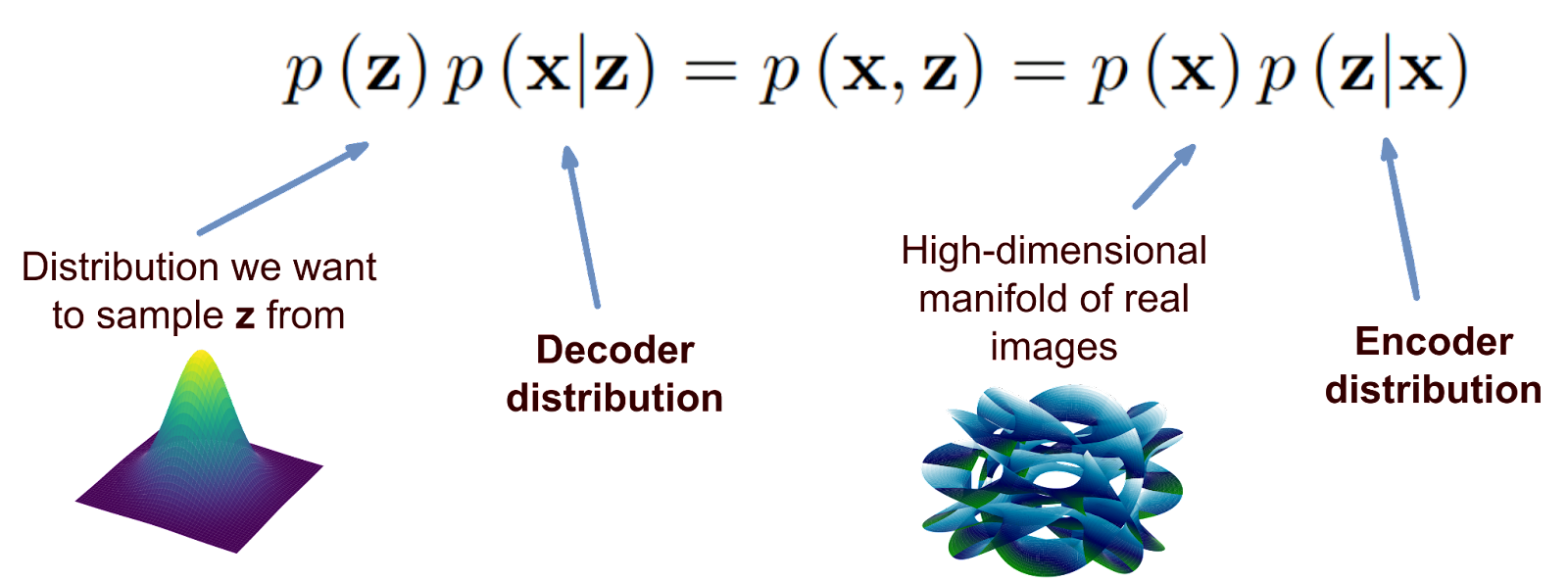
If we want to get a generative model, our main goal is to learn both p(x|z) and p(z|x). But here is the thing: in a generative model p(z) is by design simple since we need to be able to sample from it, while p(x) is, in any model, unimaginably complex since this is the distribution of real objects (images). So we cannot have both the encoder distribution p(x|z) and decoder distribution p(z|x) be simple: if, say, they both were Gaussian we’d have a Gaussian on the left but definitely something much more complicated on the right-hand side of the equation.
We need to pick one:
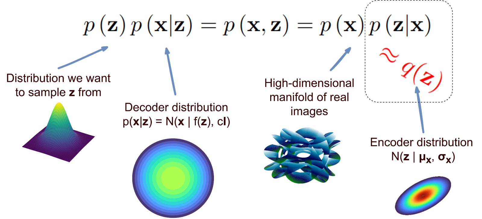
Variational autoencoders take the first option: we will assume that p(x|z) = N(x | f(z), cI) is a Gaussian distribution with mean f(z) = Decoder(z) and covariance matrix cI which is just a constant c along every axis. Thus, on the left we have a simple Gaussian p(z|x) times a simple Gaussian p(z) = N(z | 0, I), that is, another Gaussian.
What do we do on the right-hand side? We need to find a very complex distribution p(z | x). There are several different ways to do that, and variational autoencoders take the road of approximation: the encoder produces a simple distribution p(z | μx, σx), actually again a Gaussian N(z | μx, σx), but this time we cannot say that this Gaussian is the real p(z | x), we have to say that it’s an approximation:
The only thing left is how to find such an approximation. This is where the variational part comes in: variational approximations are how probability distributions are usually approximated in machine learning.
I promised not to have too much math; I lied. But you already have the basic intuition so now you can safely skip to the very end of this section and still understand everything that goes afterwards. With that said, if you are not afraid to get your hands a little dirty let us still go through the inference.
The idea of variational approximations is shown in the sequence of equations below. We start with an obvious identity, take the expectation over q(z) on both parts, and then do some transformations to break down the right-hand part into two terms, while the left-hand side does not depend on z, so the expectation simply disappears:
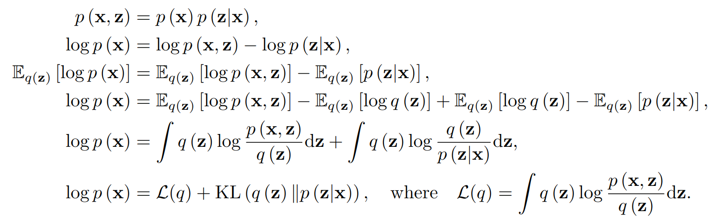
As a result, we have a constant (that is, something independent of q(z)) on the left and the sum of L(q) and the Kullback-Leibler divergence between q(z) and p(z|x) on the right, that is, a measure of how close these distributions are to each other:
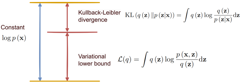
This means that we can approximate p(z|x) with q(z), i.e., minimize the divergence between them, by maximizing the first term L(q). But this first term is probably much easier to handle since it contains the joint distribution p(x, z) and not the conditional distribution p(z|x). In particular, we can now decompose it in the other way:
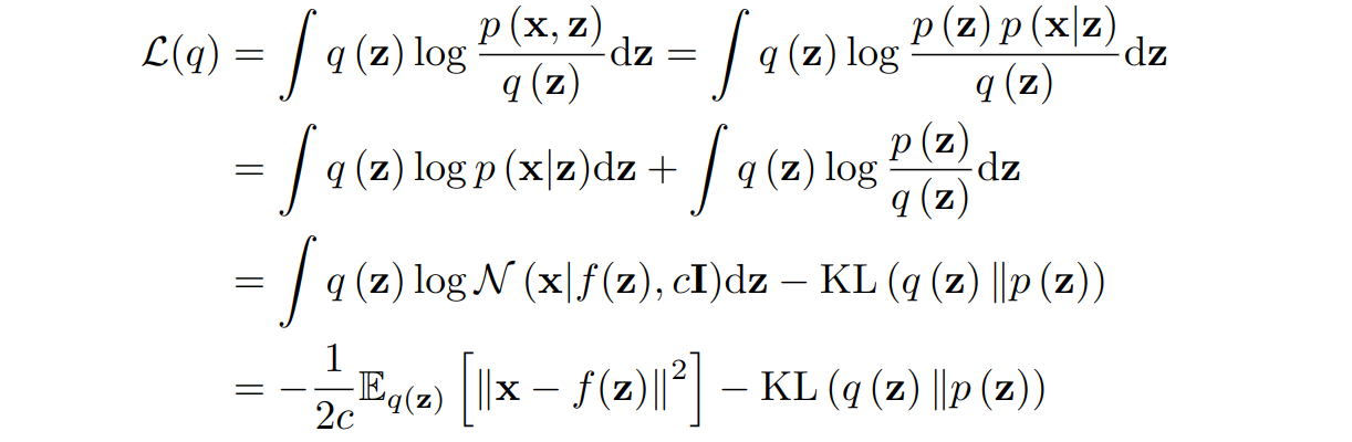
And now we have arrived at exactly the two terms that we considered in the first “intuitive” part! We need to maximize L(q), so the first term wants to make f(z) as close as possible to x, and the second term wants to make q(z) as close as possible to p(z), that is, to the standard Gaussian. Overall, we minimize exactly the sum of two terms that we had at the end of the first section:
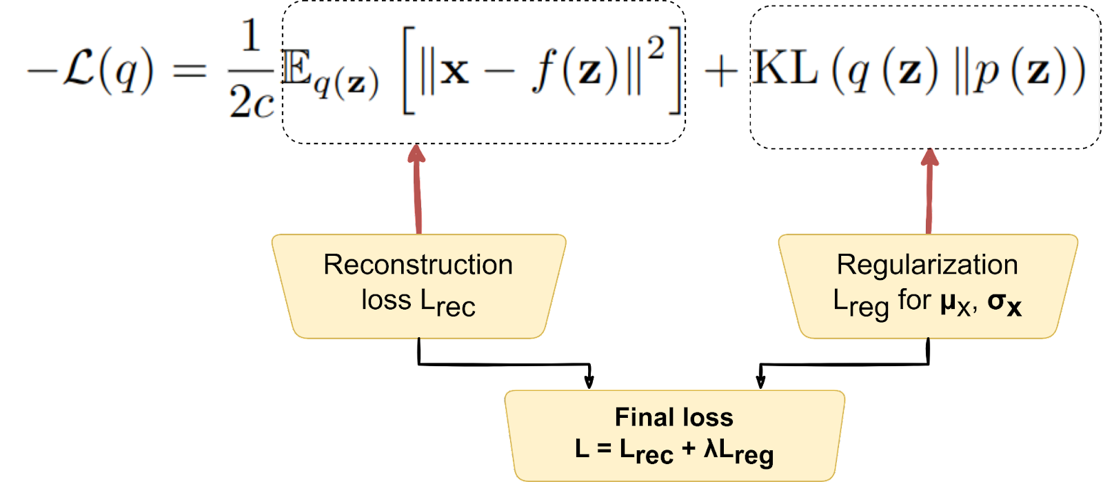
Why did we need all that math if we arrived at the exact same conclusion? Mostly because we were not sure what the reconstruction loss and the regularizer should look like. Our intuition told us that we want q(z) to be “large” but how do we formalize it exactly? And which reconstruction loss should we use? Variational approximations answer all these questions in a conceptually sound way. Moreover, they even explain the meaning of the regularization coefficient λ: turns out it’s the (inverse of) the variance for the decoder distribution. Not that it helps that much—we still need to choose c ourselves just like we needed to choose λ—but it’s always better to understand what’s going on.
By now we are almost done. I will skip the exact calculation of the regularization term: it’s tedious but straightforward and does not contain new interesting ideas; basically, you can get a rather simple exact formula in terms of μx and σx.
The only thing left is to handle the second problem: how do we train a model that has sampling in the middle?
By now, we understand the nature of the loss function in the variational autoencoder and can go back to the sampling problem:
Indeed, it is impossible to send the gradients back through the sampling process. Fortunately, we don’t need to.
The reparametrization trick comes to the rescue. The idea of this trick (we will see other versions of it in subsequent posts) is to sample a random number first from some standard distribution and then transform it into the desired distribution. In the case of Gaussians the reparametrization trick is very simple: to get a vector z from N(z | μx, σx) with a diagonal covariance matrix we can first get u from N(z | 0, I), then multiply it componentwise by σx, and then add μx to the result. The picture above in this case looks like this:
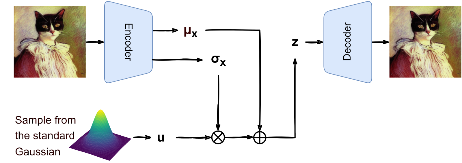
Now we can sample a mini-batch of vectors u for an input mini-batch of images and use them for training, never needing to run gradients through the sampling process.
And that’s it! Now we have the complete picture of how a variational autoencoder works, what loss function it minimizes and why, and how this loss function is related to the basic intuition of VAEs.
In this post, we have discussed the idea and implementation of VAE, a model first introduced in 2013. But these days, you don’t hear much about VAEs in the news. It’s a nice idea but is it still relevant for generative AI today?
As it turns out, VAEs are not only relevant but actually still represent one of the pillars on which the entire modern generative AI stands. Consider, for instance, the basic structure of the Stable Diffusion model (which has produced all cat images in this post):
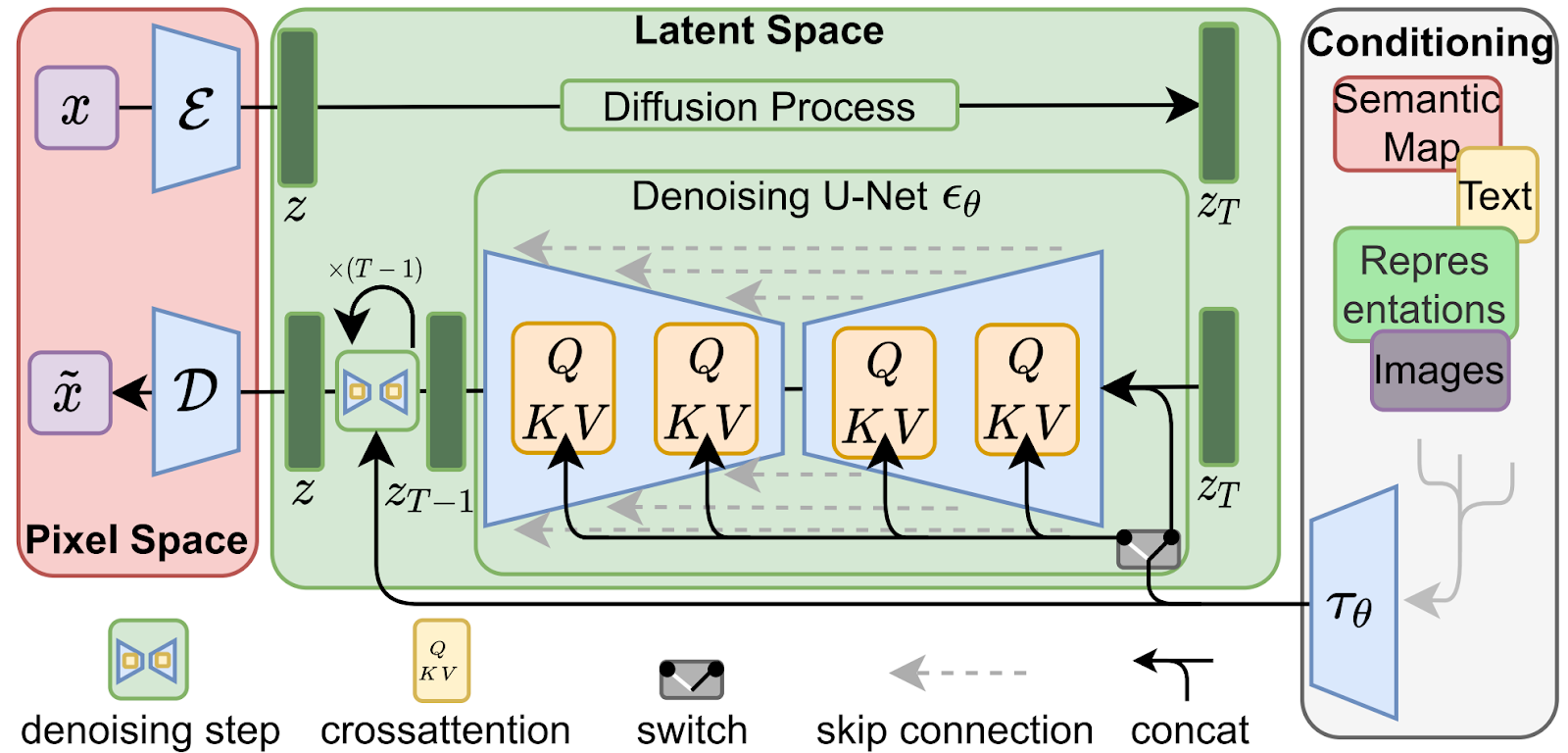
As you can see, the picture concentrates on the diffusion and denoising parts—as well it should since these are the novelties that differentiate this work from prior art. But note that all these novelties take place in the latent space of some kind of autoencoder for images, with an encoder E and decoder D mapping the codes produced by diffusion-based models into the pixel space. Where do these E and D come from? You guessed it, it’s a variational autoencoder!
But it is not the default vanilla VAE that we have discussed today. These days, it is actually either the quantized version of VAE with a discrete latent space, VQ-VAE, or its further modification with an additional discriminator, VQGAN. We will discuss these models in the next installment; until then!
Sergey Nikolenko
Head of AI, Synthesis AI