By this time, we have discussed nearly all components of modern generative AI: variational autoencoders, discrete latent spaces, how they combine with Transformers in DALL-E, and how to learn a joint latent space for images and text. There is only one component left—diffusion-based models—but it’s a big one! Today, we discuss the main idea of diffusion-based models and go over the basic diffusion models such as DDPM and DDIM. Expect a lot of math, but it will all pay off at the end.

Diffusion-based models

We have already discussed the main idea behind diffusion in machine learning in the very first, introductory post of this series. As a quick reminder, the idea is to train a model to denoise images or other objects so well that in the end, you can give it (what looks like) random noise as input and after several rounds of denoising get a realistic object.

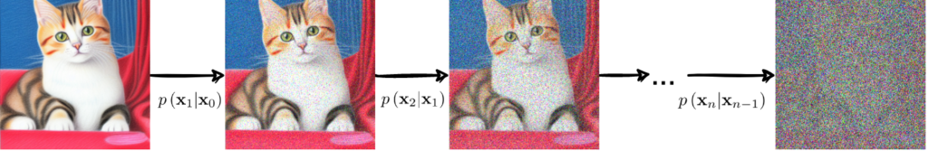
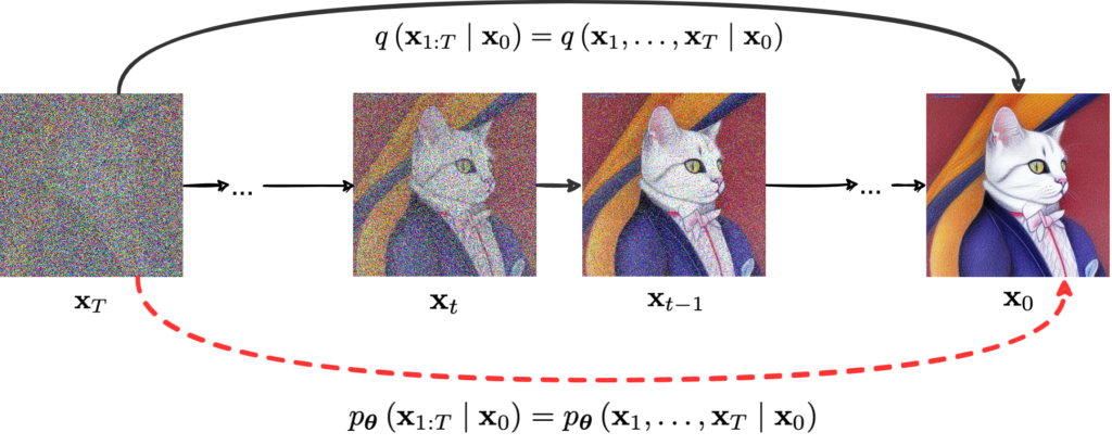
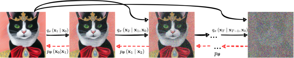
In the space of images, it would look something like this. Suppose you have some kind of a noise in mind, most probably Gaussian. This defines a probability distribution q(x_k+1|x_k), where x_k is the input image and x_k+1 is the image with added noise. Applying this distribution repeatedly, we get a Markov chain called forward diffusion that gradually adds noise until the image is completely unrecognizable:

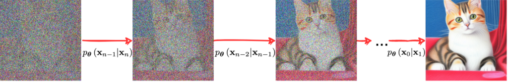
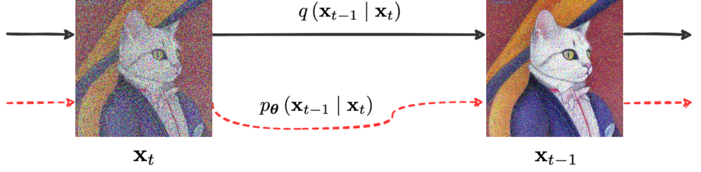
But on every step of this transformation, you add only a little bit of noise, and it is reasonable to expect that a denoising model would learn to almost perfectly get rid of it. If you get such a denoising model, again in the form of a distribution p_θ(x_k|x_k+1) with model parameters θ that should be a good approximation for the inverted q(x_k|x_k+1), you can presumably run it backwards and get the images back from basically random noise. This process is known as reverse diffusion:

However, as Woody Allen put it, “right now it’s only a notion, but I think I can get money to make it into a concept, and later turn it into an idea”. Training a denoising model straightforwardly, by using pairs of images produced by q(x_k+1|x_k) as supervision, will not get us too far: the model needs to understand the entire dynamics and make its backwards steps smarter.

Therefore, we use approximate inference to get from x_n to x₀. Since we already know variational autoencoders, I will mention that one good way to think about diffusion models is to treat them as hierarchical VAEs that chain together several feature-extracting encoders, but with additional restrictions on the encoders and decoders.

But this is where it gets mathy. The next section is not for the faint of heart, but I still include it for those of you who really want to understand how this stuff works. I will not refer to the derivation details later, so if the next section is a bit too much, feel free to skip it.

Probabilistic diffusion models: idea and derivation

Probabilistic diffusion models were introduced by Sohl-Dickstein et al. in “Deep Unsupervised Learning using Nonequilibrium Thermodynamics” (2015). As you can see from the title, it was a novel idea that went in an unexplored direction, and it had taken five years since 2015 to make it work reasonably efficiently, and a couple more years to turn it into the latent diffusion type models that we enjoy now.

Still, the basic concept remains the same. The forward diffusion process adds Gaussian noise, and the reverse diffusion model learns to restore the original image. Let’s dive into the details!

First, if we consider the noise to be Gaussian then we can get a result very similar to the reparametrization tricks we have seen earlier for VAE and dVAE: we can “compress” the whole chain into a single Gaussian. Formally, assume that q(x_t|x_t-1) is a Gaussian with variance β_t and mean that reduces x_t-1 by a factor of the square root of ɑ_t=1-β_t (this is necessary to make the process variance preserving, so that x_t would not explode or vanish), and the entire process takes T steps:

Then we can write

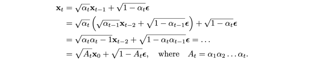
This means that the compressed distribution q(x_T|x₀) is also a Gaussian, and we know its parameters:

This makes the forward diffusion process very efficient: we can sample from q(x_T|x₀) directly, in closed form, without having to go through any intermediate steps.

It might seem that inverting Gaussians should be just as easy as stringing them together. And indeed, if our problem was to invert the Gaussian part of the process for a given x₀, it would be easy! Let’s use the Bayes formula and substitute distributions that we already know:

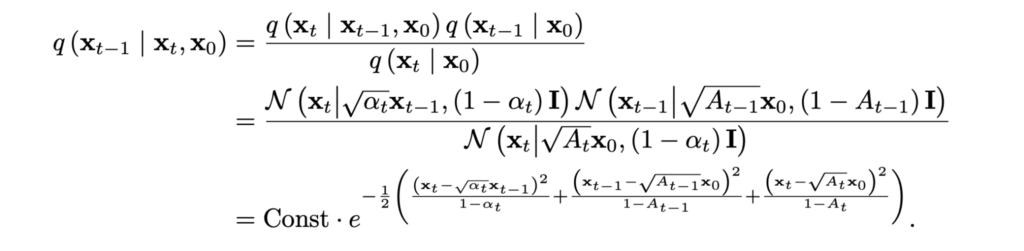
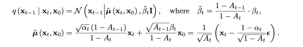
It is already clear that the new distribution is a Gaussian as well, since its density has a quadratic function of x_t-1 in the exponent. I will skip the gory details of extracting the square from this exponent, but the result is, again, a nice and clean Gaussian whose parameters we know and that we could easily sample from:

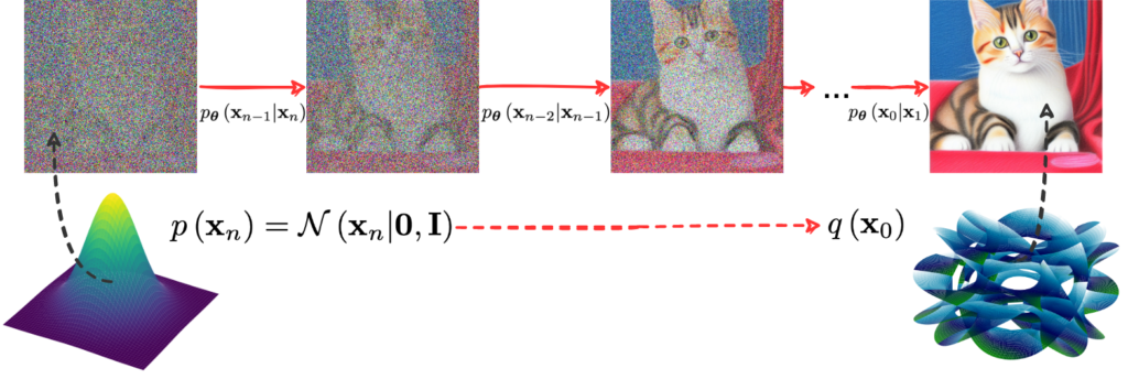
Are we done? Of course not, we are just getting started! This simple distribution is conditioned on x₀… but it is exactly q(x₀) that represents the impossibly messy distribution of, say, real life images. Ultimately we want our reverse diffusion process to reconstruct q(x₀) from a standard input at x_n; something like this:

The whole problem of training a generative model, as we have discussed many times on this blog, is to find a good representation for q(x₀), and our process so far treats it as a known quantity.

What do we do? As usual in Bayesian inference, we approximate. On every step, we want the model to be a good approximation to q(x_t|x_t-1), with no conditioning on the unknown x₀:

To get this approximation, we need a variational lower bound pretty similar to the one used in variational autoencoders and DALL-E. We will start with a bound for the global distribution  q(x_1:T|x₀) = q(x₁,…,x_T|x₀):

And then it will turn out that it decomposes into bounds for individual steps of the diffusion process.

Since we’re doing a lot of math here anyway, let us derive the variational lower bound from first principles, just like we did in the post on VAEs. We start from the obvious equality

take the expectation with respect to q(x_0:T)=q(x₀,…,x_T), and then add and subtract log q(x_1:T|x₀) = log q(x₁,…,x_T|x₀) on the right-hand side:

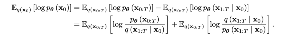
At this point, we note that the second term on the right is the KL divergence between q(x_1:T|x₀) and p_θ(x_1:T|x₀), so that’s what we want to minimize in the approximation. Since on the left-hand side we have a constant independent of x_1:T, minimizing the KL divergence with respect to q(x_1:T|x₀) is equivalent to maximizing the first term on the right, which is our bound. 

It will be more convenient to think of it as a loss function, so let’s add a minus sign in front, that is, let’s invert the fraction inside the logarithm. Then we can note that the bound decomposes nicely into the sum of individual steps; this is the last long derivation in this post (phew!):

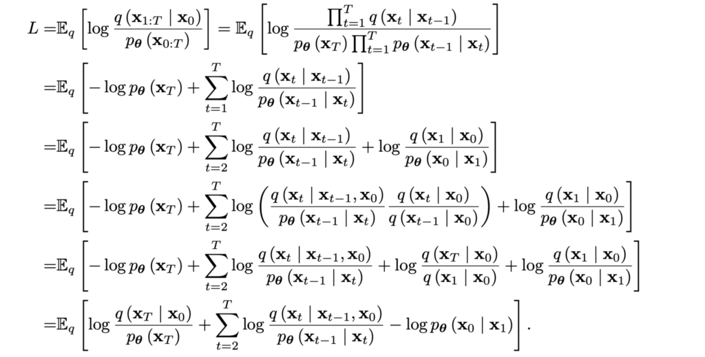
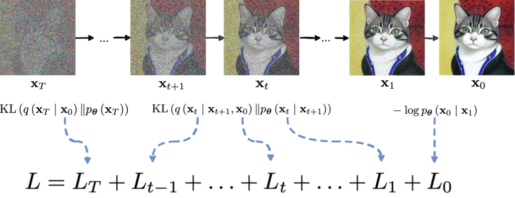
Now we see that the loss function decomposes nicely into a sum of T+1 components, and almost all of them are actually KL divergences between Gaussians:

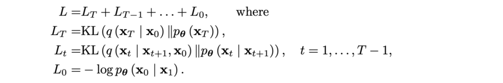
All of these components are now relatively straightforward to compute; for example, in L_t we are using the Gaussian parametrization

and trying to match its parameters with q(x_t|x_t-1, x₀). For the mean, for instance, we get

and since we know x_t during training, we can actually parametrize the noise directly rather than the mean:

I will stop the calculations here but I hope you are convinced now that this whole reverse diffusion Markov chain comes down to a closed form loss function that you can program in PyTorch and minimize. This was the main idea of the original paper by Sohl-Dickstein et al. (2015). Let us see where it has gone since then.

Denoising diffusion probabilistic models

In 2015, the original diffusion model could only be run on datasets that by now sound more like toy examples. For instance, Sohl-Dickstein et al. give examples of how their generative model fares on CIFAR-10. In the image below, (a) shows some original hold-out images from CIFAR-10, in (b) they are corrupted with Gaussian noice, (c) shows how the diffusion model can denoise the images from (b), using them as starting points for the reverse diffusion chain, and finally (d) shows new samples generated by the diffusion model:

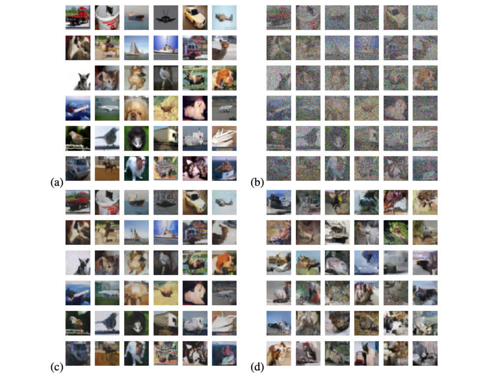
That looked somewhat promising, but perhaps not promising enough to warrant a concerted effort to develop this approach. At the time, people were just getting excited with GANs: the original work by Goodfellow was published in 2014, ProGAN (thispersondoesnotexist) would be released in 2017, and GANs would define state of the art in image generation for the next years, until they arguably ran out of steam somewhere about StyleGAN 3.

Therefore, the next stop on our way happened only five years later, in 2020, in the work “Denoising Diffusion Probabilistic Models” (DDPM) by Ho et al. They used the same basic idea and arrived at the same basic structure of the loss function; I reproduce it here in a general form since I suspect many readers have not followed through all the derivations in the previous section:

There are three different components in this loss function, two of them appearing at the ends of the chain and one that is responsible for every intermediate step. Ho et al. make the following observations and simplifications:

• they assume all forward diffusion variances β_t to be constant hyperparameters and do not train them, so there is nothing to train at all in the forward diffusion distributions q; since p_θ(x_T) is a fixed distribution that we want to sample from, this means that L_T is a constant and can be ignored;
• for the intermediate steps, they do not train the variances in p_θ(x_t|x_t+1) either, setting them to σ²I for some constant σ; they also develop the noise reparametrization mentioned above somewhat further, obtaining a simple closed form for L_t;
• finally and most importantly, they substitute a separate discrete decoder for L₀; namely, they assume that the data consists of integers from 0 to 255 scaled linearly to [-1, 1], which is a natural representation for images, and model
  
  where i goes over the pixels (components of x), μ_θ(x₁) is the independent decoder model, and the integration limits define an interval of length 1/255 on every side of x_0,i, which is a standard trick to make everything smooth and continuous.

As a result, you can substitute a different model at the last step and use a noiseless μ_θ(x₁) during test-time sampling, which extends the capabilities of the whole diffusion model significantly.

With these modifications, DDPM was able to achieve state of the art generation, comparable with the best GANs of the time. Here is a sample:

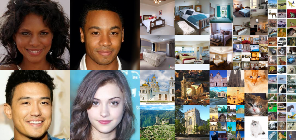
Still, that’s not quite the end of the story even for basic diffusion-based models.

Denoising Diffusion Implicit Models

The next step came very quickly after DDPMs, in the work called “Denoising Diffusion Implicit Models” (DDIM) by Song et al. (2020). They aim at the same model as DDPM, but address an important drawback of all diffusion models we have discussed so far: they are extremely slow. The generation process mirrors every step of the diffusion process, so to generate a new sample you have to go through thousands of steps (literally!), on every step we have to apply a neural network, and the steps are consecutive and cannot be parallelized. This is especially bad in contrast to the usual deep learning paradigm where it might take you a very long time to train a model but applying it is usually pretty fast: Song et al. mention that sampling from a trained GAN is over 1000x faster than sampling from a DDPM trained for the same image size.

How can we speed up this construction, which at first glance looks inherently incremental? Song et al. do it by generalizing diffusion models and DDPMs specifically. They note that the loss function we discussed above does not depend directly on the joint distribution q(x_1:T|x₀) = q(x₁,…,x_T|x₀) but only on the marginal distributions q(x_t|x₀). This means that we can reuse the exact same learning objective for a different joint distribution as long as it has the same marginals.

Song et al. define their diffusion process in terms of its reverse form:

Now we can express the forward diffusion distributions via the Bayes theorem:

Song et al. show (I promised to contain the complicated math in the first section, so I’ll skip the derivation here) that the resulting process has the same marginals, and the reverse diffusion can be trained with the same loss function and will represent an actual Markov chain:

So far it does not sound very helpful: we have extended the class of forward diffusion distributions but sampling a new image still requires going through all the reverse diffusion steps. However, the key observation here is that instead of approximating the random noise ε_t that gets us from x_t to x_t+1, we are now approximating the random noise ε_t that is mixed with x₀ to obtain x_t+1. 

This process, in essence, means that when we are going in the reverse direction, we are approximating the direction not to x_t, but directly to x₀, and make a step in that direction. Here is an illustration for the difference:

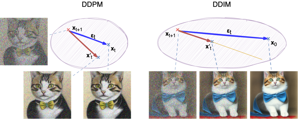
A DDPM model is trying to approximate the step from x_t+1 to x_t, failing somewhat and getting a worse image. A DDIM model is trying to approximate the direction all the way from x_t+1 to x₀; naturally, it fails a little and if it tried to go all the way to x₀ it would miss by a lot so it makes a small step in the approximate direction. It is hard to say which method is doing a better job at the approximation itself, but there is an important benefit to the DDIM scheme in terms of performance.

Since now ε_t and the dependence on x₀ are disentangled, ε_t is just a Gaussian noise variance, and we can jump over several steps in the process, getting from x_t to x_t+k in a single step with correspondingly increased ε! One can train a model with a large number of steps T but sample only a few of them in the generation part, which speeds things up very significantly. Naturally, the variance will increase, and the approximations will get worse, but with careful tuning this effect can be contained.

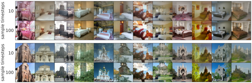
Song et al. achieve 10x to 100x speedups compared to DDPM, with insignificant loss in quality:

Moreover, DDIMs also have a generation process that does not need to be stochastic! Song et al. suggest setting the variance hyperparameter in the reverse diffusion chain to zero during generation. This means that a latent code in the space of x_T corresponds to exactly one image, and now we can expect DDIMs to behave in the same way as other models that train latent representations (compare, e.g., our previous post), including, for instance, interpolations in the latent space:

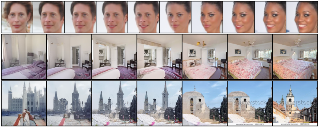
Note that DDPMs could not do interpolations because a latent code x_T would have a huge amount of noise added to it during the reverse diffusion process; it wasn’t really a “code” for anything, just a starting point for the Markov chain.

Conclusion

Today, we have introduced the basics of diffusion models in machine learning. This field started in 2015, and its basic idea of learning gradual denoising transformations was preserved in later developments: DDPMs made several improvements that allowed to scale diffusion models up, and DDIMs increased the performance of the generation process and made it deterministic, which opened up a number of new possibilities.

There is basically only one step left before we get to the cutting edge models such as Stable Diffusion and DALL-E 2. Next time, we will take this step; stay tuned!

Sergey Nikolenko
Head of AI, Synthesis AI