Last time, we discussed one of the models that have made modern generative AI possible: variational autoencoders (VAE). We reviewed the structure and basic assumptions of a VAE, and by now we understand how a VAE makes the latent space more regular by using distributions instead of single points. However, the variations of VAE most often used in modern generative models are a little different: they use discrete latent spaces with a fixed vocabulary of vectors. Let’s see what that means and how it can help generation!

Continuous and Discrete Latent Spaces

We have already discussed latent spaces in both the introductory post and the post on variational autoencoders but this time we have a slightly different spin. In general, an autoencoder is compressing the high-dimensional input (say, an image) into a low-dimensional representation, i.e., into a relatively short vector of numbers whose dimension is in the hundreds rather than millions:

If the autoencoder is designed well, this may result in a latent space where certain directions correspond to specific properties of the image. For instance, if we are compressing cat images then one axis may correspond to the cat’s color and another to the overall style of the image:

Naturally, in reality these directions would not necessarily coincide with coordinate axes and may be hard to find. There’s no preference for a regular autoencoder architecture (say, a VAE) to find a latent space with well-defined directions. In fact, it is easy to see that the latent space may undergo rather complicated transformations with no change in the model complexity: there is usually no difference between learning an encoder Enc and decoder Dec and learning an encoder f○Enc and decoder Dec○f⁻¹ for some invertible transformation f.

This is an appealing picture, but it’s not as easy to obtain, and, moreover, it’s not really how we think about styles and picture descriptions. We are verbal creatures, and when I want to get a picture of a black cat I don’t have a real number associated with its “blackness”, I just want a cat with a discrete “black” modifier, just like I might want a “white” modifier. A black and white cat for me is not a number that reflects the percentage of white hair but most probably just a separate “black and white” modifier that turns out to be in a rather complex relationship with the “black” and “white” modifiers.

Can we try to reflect this intuition in an autoencoder latent space? We could imagine a latent space that has a vocabulary of “words” and decodes combinations of these words into images. Something like this:

This looks much more “human-like”, and the last few years of generative AI have indeed proven this approach to be significantly more fruitful. Its best feature is the ability to use autoregressive generative models for discrete latent representations. For example, the famous Transformers, in particular the GPT family, can be applied to produce latent space “words” just as well as they produce real words in their natural language applications, but they would be much harder to adapt to components of continuous latent vectors.

But the discrete latent space approach comes with its own set of problems, both technical and conceptual. In the rest of this post, we will go through two models that successfully solved these problems and thus became foundational for modern generative AI.

VQ-VAE: Vector Quantized VAE

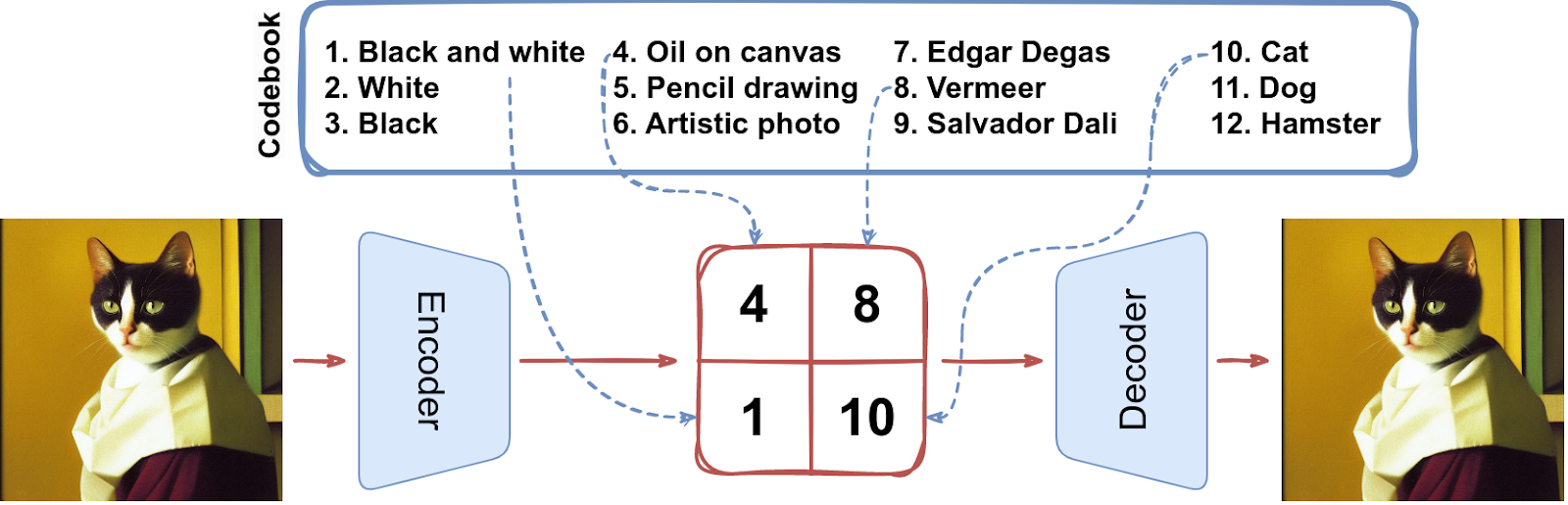
The first model that successfully managed to construct a discrete latent space at a scale sufficient for general-purpose images was Vector Quantized VAE (VQ-VAE) introduced back in 2017 by DeepMind researchers (van den Oord et al., 2017). Its basic idea is exactly as we have discussed: VQ-VAE finds a finite vocabulary (codebook) and encodes images as fixed sets (tensors) of discrete codes:

It turns out that it’s not a good idea to make the encoder do actual classification over the codebook vectors. Therefore, here’s what we want to happen:

• the encoder, as usual, takes an image x as input and produces a set of latent vectors Enc(x); a slight difference with our previous settings is that now the encoder produces a whole set of vectors (usually formalized as a three-dimensional tensor, i.e., a matrix of vectors), but mathematically it’s equivalent to slicing a single output vector;
• for every latent vector, we find the nearest codebook vector in the latent space and replace it with this codebook vector; the resulting code consists only of codebook vectors;
• the decoder receives as input the tensor of vectors, with the same dimensions as the encoder had produced, but actually the latent code is now discrete: while each component of the latent code is still a continuous vector of real numbers, there’s now only a finite number of possibilities for each of the vectors.

Here’s an illustration (I only show how one vector is chosen but the procedure is the same for each of them):

At this point, some readers might be wondering: there’s now only a finite number of latent codes in total! There is no boundless generation, characteristic for natural languages where we can have texts as long as we like. Won’t that severely limit the models? Well, a realistic size of the latent code tensor is something like 32×32 with, say, 8192 codebook vectors (the numbers are taken from the original DALL-E model). There are two ways to look at these numbers. On the one hand, this amounts to 8192^32×32 = 2⁴⁰⁹⁶⁰ possibilities while the number of atoms in the Universe is less than 2³⁰⁰, so it looks like we are covered. On the other hand, this is equivalent to compressing every possible image of size 256×256 (the dimensions of original DALL-E) into 40960 bits, i.e., a bit more than 5 kilobytes of data, which means that we will need quite a compressing tool. Both views are valid: modern autoencoder-based models are indeed very impressive in their ability to compress images into latent representations, but the diversity of their outputs does not bound our imagination too much.

There are two questions remaining. First, how do we train the encoder and decoder networks? It looks like we have the same problem as VAE had: just like VAE had sampling in the middle, VQ-VAE has a piecewise constant operation (taking the nearest neighbor), and the gradients cannot flow back through this operation. And second, how do we learn the codebook vectors?

At this point, I will show a picture from the original VQ-VAE paper; it always comes up in these discussions, and we need its notation to discuss the VQ-VAE objective, so you need to see it too:

This picture mostly illustrates the idea of a discrete latent space with codebook vectors that we have already discussed. But it also shows the solution to the first problem: VQ-VAE simply copies the gradients (red line) from the decoder to the encoder, that is, the gradient of the loss function with respect to the tensor of codebook vectors is assumed to be its gradient with respect to Enc(x). This is an approximation, of course, and one can remove it with a more involved construction (a discrete VAE with the Gumbel-Softmax trick that we will explain in a later post on DALL-E), but for now it will have to do.

As for the second problem, it brings us to the VQ-VAE training objective. Here is the loss function as defined by van den Oort et al. (2017):

This formula sure begs for a detailed explanation. Let’s first go through all the notation step by step and then summarize:

• z_e(x) and z_q(x) are two latent representations for an image x produced by the encoder: z_e is the output of the decoder and z_q is the codebook representation after replacing each vector with its nearest codebook neighbor (this notation is illustrated in the image above); the first term is responsible for training the decoder network;
• p(ᐧ|z) is the distribution of reconstructed images after the decoder given the latent code; we want the reconstruction to be good so we maximize the likelihood of the original image x given its latent code z_q(x) that serves as input for the decoder;
• sg[ᐧ] is the stopgradient operator; it is defined as the identity during the forward pass (when we compute the objective function L) and zero during the backward pass (when we compute the gradient ∇_wL);
• therefore, the second term means that we want to bring each codebook vector e closer to the latent codes z_e(x) that choose it as its nearest neighbor; this term is responsible for training the codebook;
• the third term is the opposite: it brings z_e(x) closer to their corresponding codebook vectors; in effect, the second and third term together do a kind of clustering of latent codes z_e(x) around their corresponding codebook vectors; the hyperparameter ???? can balance the two terms although the authors say that the results don’t change for  ???? at least from 0.1 to 2.0;
• finally, the encoder network is trained with the first and third terms where it occurs in the form of z_e(x).

In the illustration below, I show the components of the objective function and what their contributions are in the latent space (on top) and on learning the weights of the encoder and decoder networks (at the bottom):

Interestingly, the original paper has a typo in its main formula repeated in countless blog post explanations: the authors forgot the minus sign in front of the likelihood so in their training objective the first term should be maximized and the other two minimized. Naturally, it’s just a typo, and all working VQ-VAE implementations get it right, but it’s funny how these things can get propagated.

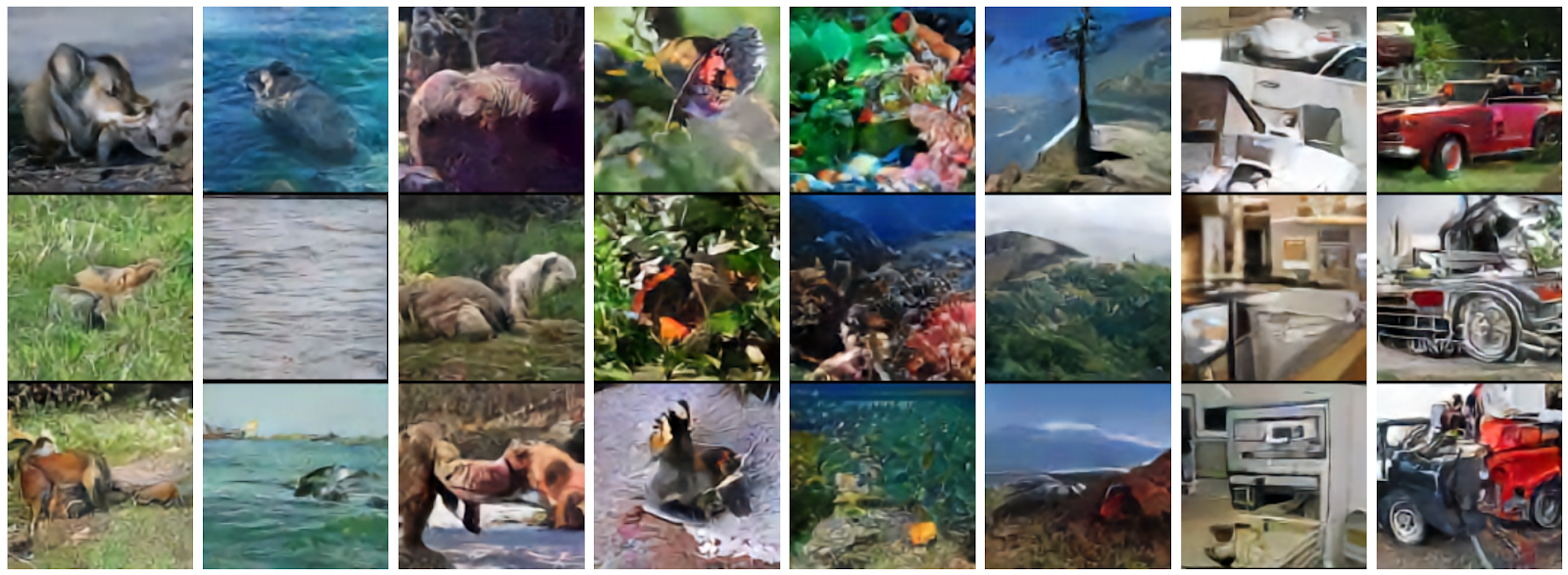
That’s it for VQ-VAE. The original model predated Transformers so it could not use them for latent code generation but they used a different autoregressive model which was state of the art at the time: PixelCNN (van den Oord et al., 2016; Salimans et al., 2017). PixelCNN itself originated as a model for generating pictures, but generating a high-resolution image autoregressively, pixel by pixel, is just way too slow (see also my first post in this series). But it’s just fine for generating a set of 32×32 codebook tokens! The original VQ-VAE, trained on ImageNet with a separate PixelCNN trained to generate latent codes, produced impressive results by 2017 standards:

The next step was VQ-VAE 2 that still used PixelCNN for latent codes but moved to a hierarchical structure, generating a small top-level representation and then a more detailed bottom-level representation conditioned on the top level result:

VQ-VAE 2 produced excellent results. When it came out, in 2019, in the wake of ProGAN (you may have heard of it as “This person does not exist”) everybody was comparing generation abilities on a dataset of high-dimensional celebrity photos, and VQ-VAE 2 did not disappoint:

But we still have some way to go before DALL-E 2 and Stable Diffusion, even in terms of the underlying autoencoders. The next step for VQ-VAE was to turn it into a GAN…

VQ-GAN: Add a Discriminator to the Mix

VQ-VAE and VQ-VAE 2 left us with some very good generation via discrete latent codes but the codes were still produced by a PixelCNN model. Naturally, we’d like to generate these codes with a Transformer-based architecture, at least because it’s much better at handling global dependencies: a Transformer does not even have the notion of a “long” or “short” dependency, it always attends to every previously generated token.

It was only natural that the next step would be to use a Transformer to generate the codes. So in the autoencoder part, we would have something similar to VQ-VAE, and then the Transformer would serve as the autoregressive model to generate the codes:

So in this approach, an image becomes a sequence of codebook vectors, and the Transformer does what it does best: learns to generate sequences. 

One of the problems here is that we need to learn a very rich and expressive codebook. So instead of using just a straightforward reconstruction loss, VQ-GAN (Esser et al., 2020) adds a patch-based discriminator that aims to distinguish between (small patches of) real and reconstructed images, and the loss becomes a perceptual loss, i.e., the difference between features extracted by some standard convolutional network (Zhang et al., 2018). This means that the discriminator now takes care of the local structure of the generate image, and the perceptual loss deals with the actual content.

In total, the losses for our autoencoder might look something like this:

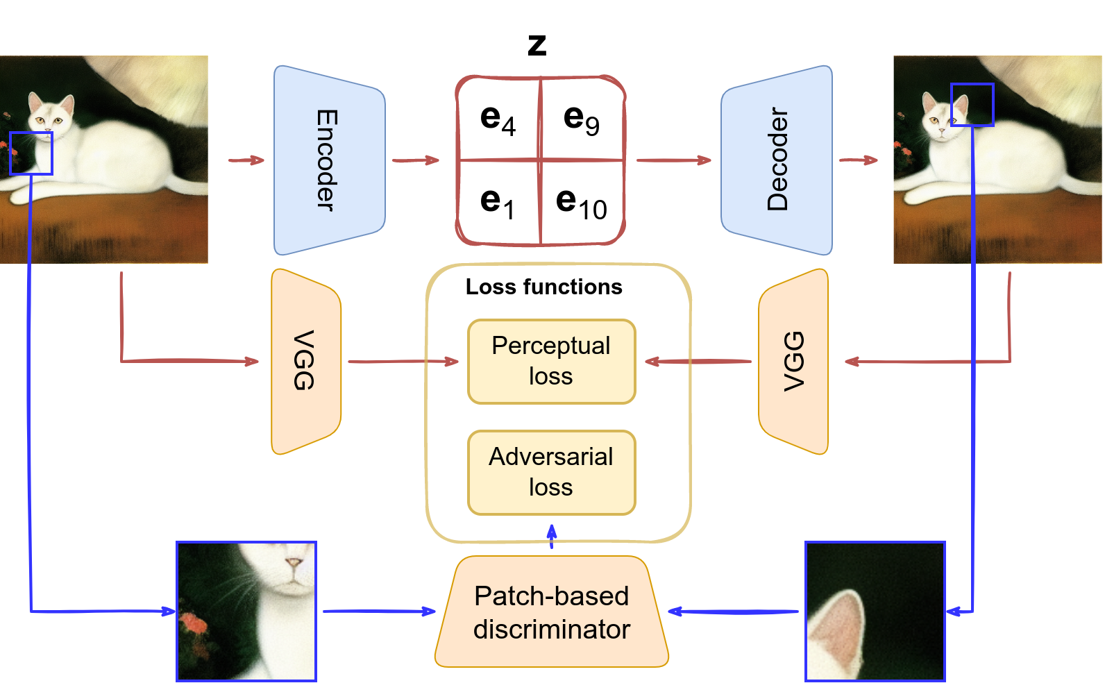
And with this, we are ready to see the overview of the whole architecture as it is shown in the original VQ-GAN paper (Esser et al., 2020):

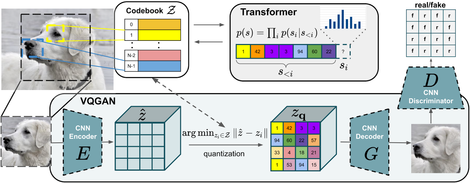
Just like a regular VQ-VAE, an image is represented with a sequence of discrete codebook vectors, but now the reconstruction is ensured by a combination of perceptual and adversarial losses, and the codes are produced by a Transformer.

VQ-GAN could produce better images on the basic ImageNet—here are some first rate goldfinches compared to other approaches:

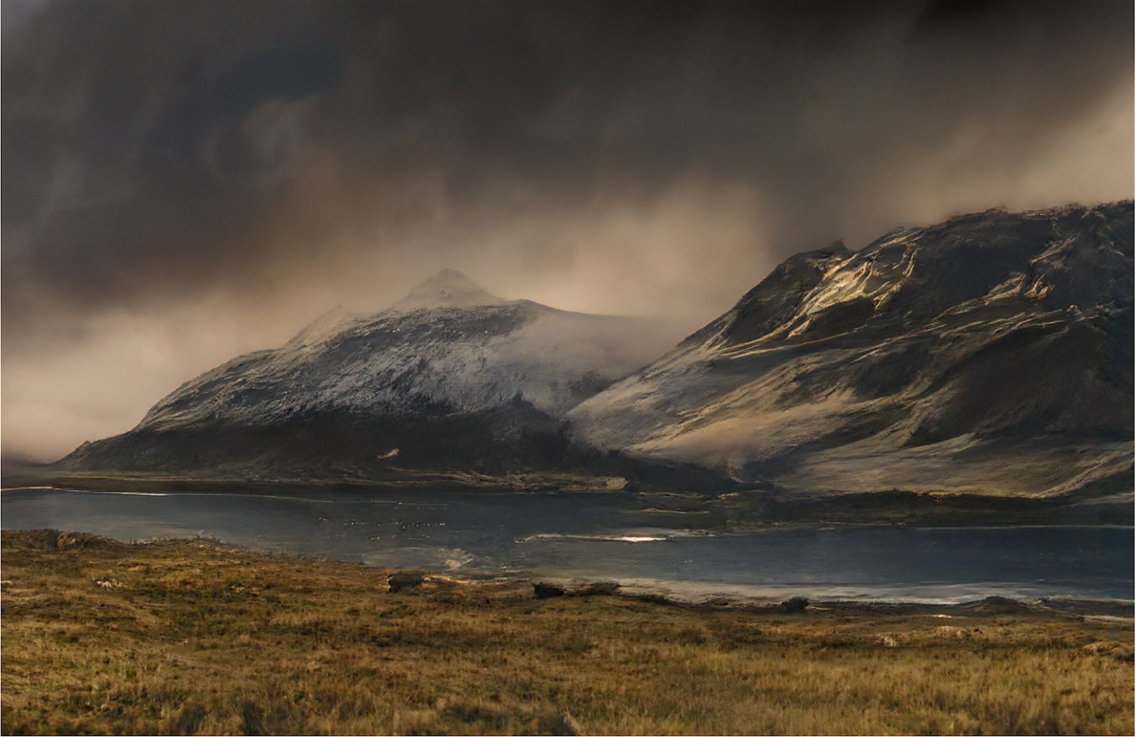
But a major point about VQ-GAN was that it could scale to far higher resolutions. Here is a sample landscape (originally 1280×832 pixels) generated by the VQ-GAN from a semantic layout, i.e., from a rough segmentation map showing where the sky, land, mountains, and grass should be:

As a result, VQ-GAN, like virtually every method we discuss, defined the state of the art for image generation when it was introduced. We have to stop here for now, but our story is far from over…

Conclusion

In this post, we have discussed the notion of a discrete latent space, where images are compressed to sequences of tokens (“words”) instead of continuous vectors. This makes it far easier to train a good generative model since generating sequences is the bread and butter of many autoregressive models. The original VQ-VAE family used PixelCNN as this intermediate autoregressive model, but as soon as Transformers appeared it became clear that they are a great fit for this task, and VQ-GAN managed to make it work.

At this point, we are ready to put several things together and discuss not just an image generation/reconstruction model but a real text-to-image model, where (spoiler alert) the Transformer will generate a sequence of discrete latent space tokens starting with a natural language text prompt. So next time, get ready for DALL-E!

Sergey Nikolenko
Head of AI, Synthesis AI