Previously on this blog, we have discussed the data problem: why machine learning may be hitting a wall, how one-shot and zero-shot learning can help, how come reinforcement learning does not need data at all, and how unlabeled datasets can inform even supervised learning tasks. Today, we begin discussing our main topic: synthetic data. Let us start from the very beginning: how synthetic data was done in the early days of computer vision…

A brief intro to synthetic data

Let me begin by reminding the general pipeline of most machine learning model development processes:

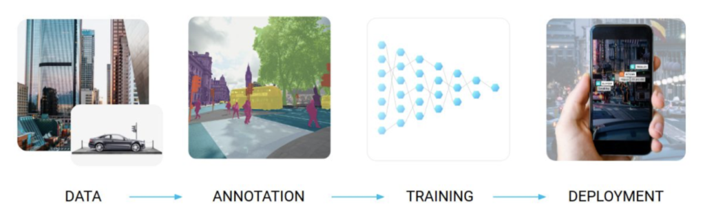
Synthetic data is an important approach to solving the data problem by either producing artificial data from scratch or using advanced data manipulation techniques to produce novel and diverse training examples. The synthetic data approach is most easily exemplified by standard computer vision problems, and we will do so in this post too, but it is also relevant in other domains.

In basic computer vision problems, synthetic data is most important to save on the labeling phase. For example, if you are solving the segmentation problem it is extremely hard to produce correct segmentation masks by hand. Here are some examples from the Microsoft COCO (Common Objects in Context) dataset:

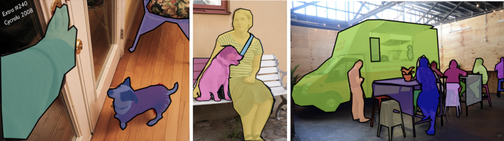
You can see that the manually produced segmentation masks are rather rough, and it is very expensive to make them much better if you need a large-scale dataset as a result.

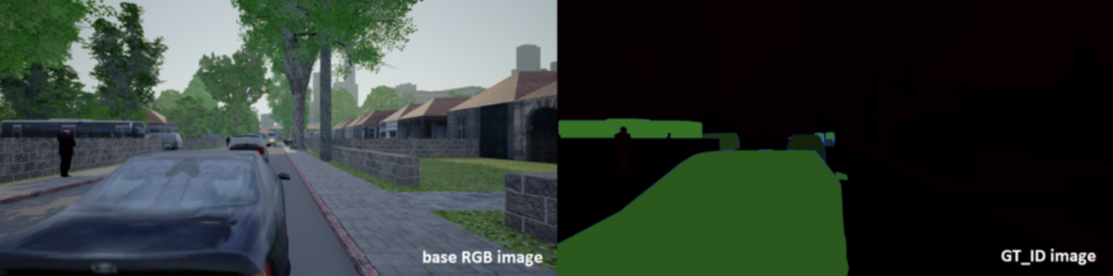
But suppose that all these scenes were actually 3D models, rendered in virtual environments with a 3D graphics engine. In that case, we wouldn’t have to painstakingly label every object with a bounding box or, even worse, a full silhouette: every pixel would be accounted for by the renderer and we would have all the labeling for free! What’s more, the renderer would provide useful labeling which is impossible for humans and which requires expensive hardware to get in reality, such as, e.g., depth maps (distance to camera) or surface normals. Here is a sample from the ProcSy dataset for autonomous driving: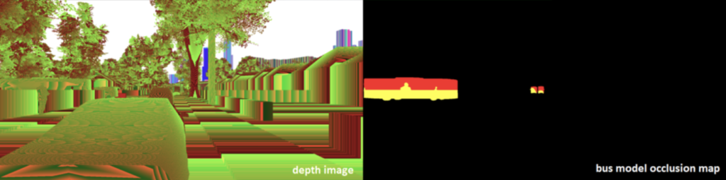

We will speak a lot more about synthetic data in this blog, but for now let us get on to the main topic: how synthetic data started its journey and what its early days looked like.

The first steps: line drawings as synthetic data

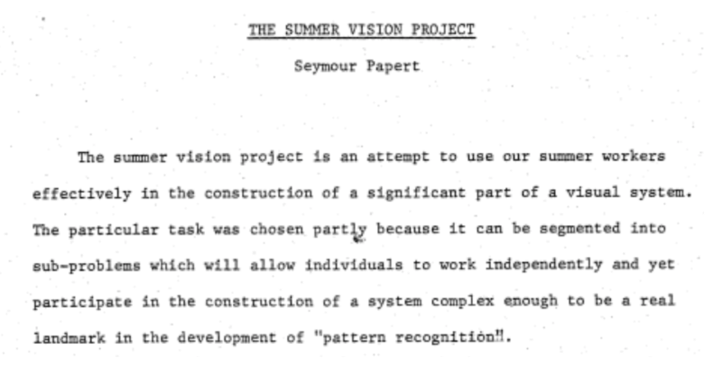
Computer vision started as a very ambitious endeavour. The famous “Summer Vision Project” by Seymour Papert was intended for summer interns and asked to construct a segmentation system, in 1966:

Back in the 1960s and 1970s, usable segmentation on real photos was very hard to achieve. As a result, people turned to… synthetic data! I am not kidding, synthetic images in the form of artificial drawings are all over early computer vision.

Consider, for example, the line labeling problem: given a picture with clearly depicted lines, mark which of the lines represent concave edges and which are convex. Here is a sample picture with this kind of labeling for two embedded parallelepipeds, taken from the classic paper by David Huffman, Impossible Objects as Nonsense Sentences:

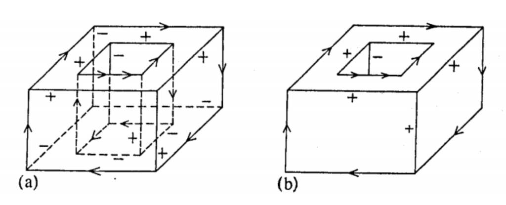
Figure (a) on the left shows a fully labeled “X-ray” image, and figure (b) shows only the visible part, but still fully labeled. And here is an illustration of a similar but different kind of labeling, this time from another classic paper by Max Clowes, On Seeing Things:

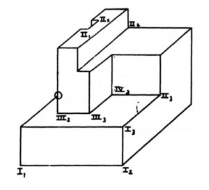
Here Clowes distinguishes different types of corners based on how many edges form them and what kind of edges (concave or convex) they are. So basically it’s the same problem: find out the shape of a polyhedron defined as a collection of edges projected on a plane, i.e., shown as a line drawing.

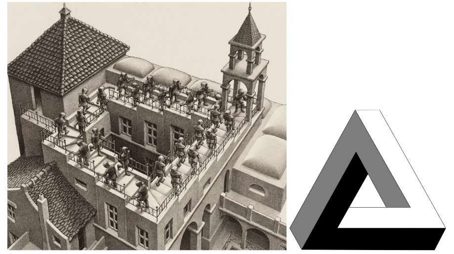
Both Huffman and Clowes work (as far as I understand, independently) towards the goal of developing algorithms for this problem. They address it primarily as a topological problem, use the language of graph theory and develop conditions under which a 2D picture can correspond to a feasible 3D scene. They are both fascinated with impossible objects, 2D drawings that look realistic and satisfy a lot of reasonable necessary conditions for realistic scenes but at the same time still cannot be truly realized in 3D space. Think of M.C. Escher’s drawings (on the left, a fragment from “Ascending and descending”) or the famous Penrose triangle (on the right):

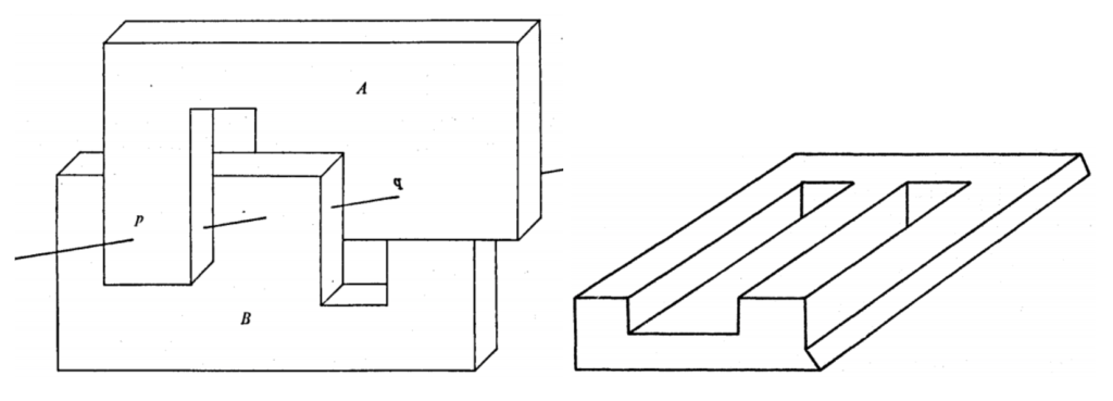
And here are two of the more complex polyhedral shapes, the one on the left taken from Huffman and on the right, from Clowes. They are both impossible but it’s not so easy to spot it by examining local properties of their graphs of lines:

But what kind of examples did Huffman and Clowes use for their test sets? Well, naturally, it proved to be way too hard for the computer vision of the 1960s to extract coherent line patterns like these from real photographs. Therefore, this entire field was talking about artificially produced line drawings, one of the first and simplest examples of synthetic data in computer vision.

Synthetic data for a quantitative comparison

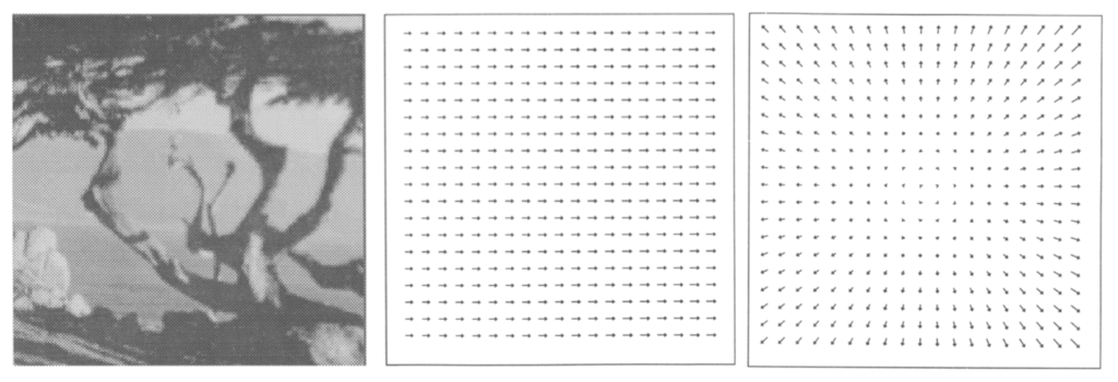
In the early days of computer vision, many problems were tackled not by machine learning but by direct attempts to develop algorithms for specific tasks. Let us take as the running example the problem of measuring optical flow. This is one of the basic low-level computer vision problems: estimate the distribution of apparent velocities of movement along the image. Optical flow can help find moving objects on the image or estimate (and probably subtract) the movement of the camera itself, but its most common use is for stereo matching: by computing optical flow between images taken at the same time from two cameras, you can match the picture in stereo and then do depth estimation and a lot of scene understanding. In essence, optical flow is a field of vectors that estimate the movement of every pixel between a pair of images. Here is an example (taken from here):

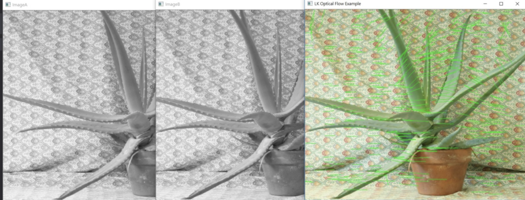
The example above was produced by the classical Lucas-Kanade flow estimation algorithm. Typical for early computer vision, this is just an algorithm, there are no parameters to be learned from data and no training set. In their 1981 paper, Lucas and Kanade do not provide any quantitative estimates for how well their algorithm works, they just give several examples based on a single real world stereo pair. Here it is, by the way: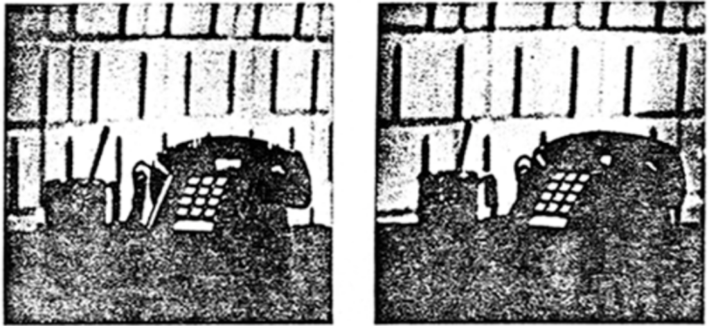

And this is entirely typical: all early works on optical flow estimation develop and present new algorithms but do not provide any means for a principled comparison beyond testing them on several real examples.

When enough algorithms had been accumulated, however, the need for an honest and representative comparison became really pressing. For an example of such a comparison, we jump forward to 1994, to the paper by Barron et al. called Performance of Optical Flow Techniques. They present a taxonomy and survey of optical flow estimation algorithms, including a wide variety of differential (such as Lucas-Kanade), region-based, and energy-based methods. But to get a fair experimental comparison, they needed a test set with known correct answers. And, of course, they turned to synthetic data for this. They concisely sum up the pluses and minuses of synthetic data that remain true up to this day:

The main advantages of synthetic inputs are that the 2-D motion fields and scene properties can be controlled and tested in a methodical fashion. In particular, we have access to the true 2-D motion field and can therefore quantify performance. Conversely, it must be remembered that such inputs are usually clean signals (involving no occlusion, specularity, shadowing, transparency, etc.) and therefore this measure of performance should be taken as an optimistic bound on the expected errors with real image sequences.

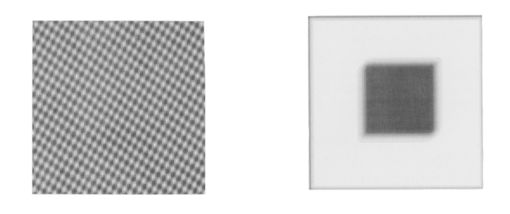
For the comparison, they used sinusoidal inputs and a moving dark square over a bright background:

They also used synthetic camera motion: take a still real photograph and start cropping out a moving window over this image, and you get a camera moving perpendicular to its line of sight. And if you take a window and start expanding it, you get a camera moving outwards:

These synthetic data generation techniques were really simple and may seem naive by now, but they did allow for a reasonable quantitative comparison: it turned out that even on such seemingly simple inputs the classical optical flow estimation algorithms gave very different answers, with widely varying accuracy.

Conclusion

Today, we saw two applications of synthetic data in early computer vision. First, simple line drawings suffice to present an interesting challenge for 3D scene understanding, even when interpreted as precise polyhedra. Second, while classical algorithms for low-level computer level problems almost never involved any learning of parameters, to make a fair comparison you need a test set with known correct answers, and this is exactly where machine learning can step up. But stay tuned, that’s not all, folks! See you next time!

Sergey Nikolenko
Head of AI, Synthesis AI