Welcome back, everybody! It’s been a while since I finished the last series on object detection with synthetic data (here is the series in case you missed it: part 1, part 2, part 3, part 4, part 5). So it is high time to start a new series. Over the next several posts, we will discuss how synthetic data and similar techniques can drive model performance and improve the results. We will mostly be talking about computer vision tasks. We begin this series with an explanation of data augmentation in computer vision; today we will talk about simple “classical” augmentations, and next time we will turn to some of the more interesting stuff.

Data Augmentation in Computer Vision: The Beginnings

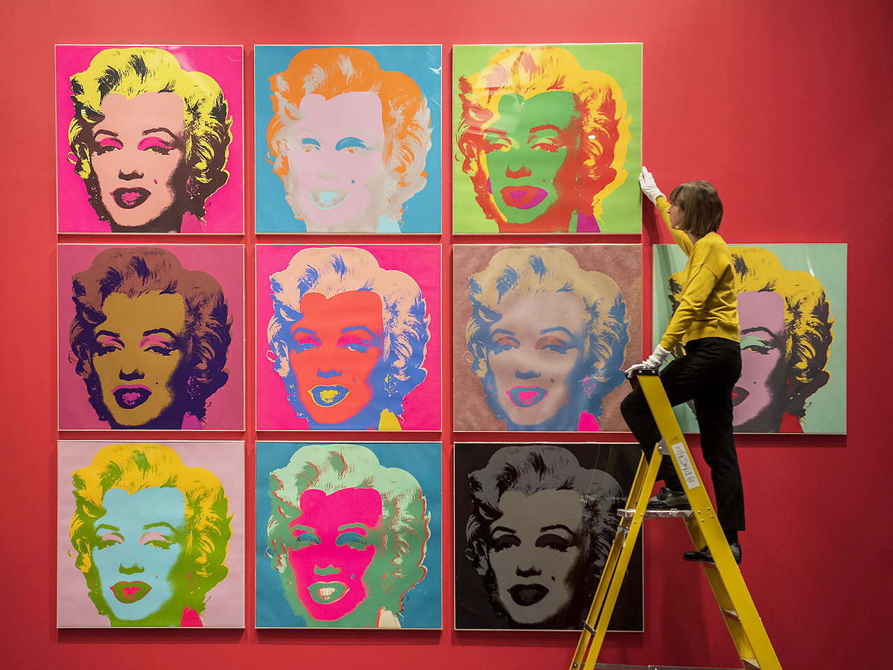
Let me begin by taking you back to 2012, when the original AlexNet by Alex Krizhevsky, Ilya Sutskever, and Geoffrey Hinton (paper link from NIPS 2012) was taking the world of computer vision by storm. AlexNet was not the first successful deep neural network; in computer vision, that honor probably goes to Dan Ciresan from Jurgen Schmidhuber’s group and their MC-DNN (Ciresan et al., 2012). But it was the network that made the deep learning revolution happen in computer vision: in the famous ILSVRC competition, AlexNet had about 16% top-5 error, compared to about 26% of the second best competitor, and that in a competition usually decided by fractions of a percentage point!

Let’s have a look at the famous figure depicting the AlexNet architecture in the original paper by Krizhevsky et al.; you have probably seen it a thousand times:

I want to note one little thing about it: note that the input image dimensions on this picture are 224×224 pixels, while ImageNet actually consists of 256×256 images. What’s the deal with this?

The deal is that AlexNet, already in 2012, had to augment the input dataset in order to avoid overfitting. Augmentations are transformations that change the input data point (image, in this case) but do not change the label (output) or change it in predictable ways so that one can still train the network on augmented inputs. AlexNet used two kinds of augmentations:

• horizontal reflections (a vertical reflection would often fail to produce a plausible photo) and
• image translations; that’s exactly why they used a smaller input size: the 224×224 image is a random crop from the larger 256×256 image.

With both transformations, we can safely assume that the classification label will not change. Even if we were talking about, say, object detection, it would be trivial to shift, crop, and/or reflect the bounding boxes together with the inputs &mdash that’s exactly what I meant by “changing in predictable ways”. The resulting images are, of course, highly interdependent, but they still cover a wider variety of inputs than just the original dataset, reducing overfitting. In training AlexNet, Krizhevsky et al. estimated that they could produce 2048 different images from a single input training image.

What is interesting here is that although ImageNet is so large (AlexNet trained on a subset with 1.2 million training images labeled with 1000 classes), modern neural networks are even larger (AlexNet has 60 million parameters), and Krizhevsky et al. have the following to say about their augmentations: “Without this scheme, our network suffers from substantial overfitting, which would have forced us to use much smaller networks.”

AlexNet was not even the first to use this idea. The above-mentioned MC-DNN also used similar augmentations even though it was indeed a much smaller network trained to recognize much smaller images (traffic signs). One can also find much earlier applications of similar ideas: for instance, Simard et al. (2003) use distortions to augment the MNIST training set, and I am far from certain that this is the earliest reference.

Simple Augmentations Today

In the previous section, we have seen that as soon as neural networks transformed the field of computer vision, augmentations had to be used to expand the dataset and make the training set cover a wider data distribution. By now, this has become a staple in computer vision: while approaches may differ, it is hard to find a setting where data augmentation would not make sense at all.

To review what kind of augmentations are commonplace in computer vision, I will use the example of the Albumentations library developed by Buslaev et al. (2020); although the paper was only released this year, the library itself had been around for several years and by now has become the industry standard.

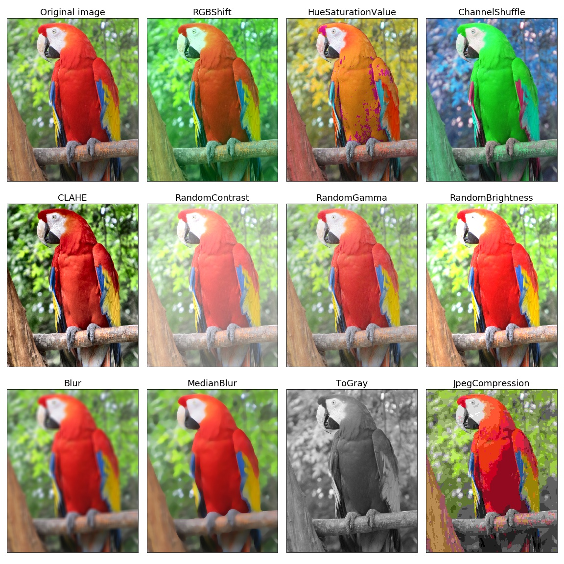
The obvious candidates are color transformations. Changing the color saturation or converting to grayscale definitely does not change bounding boxes or segmentation masks:

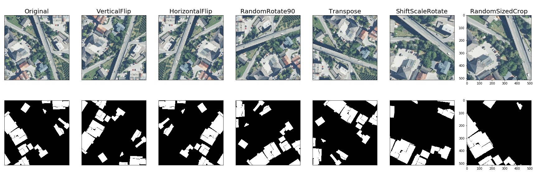
The next obvious category are simple geometric transformations. Again, there is no question about what to do with segmentation masks when the image is rotated or cropped; you simply repeat the same transformation with the labeling:

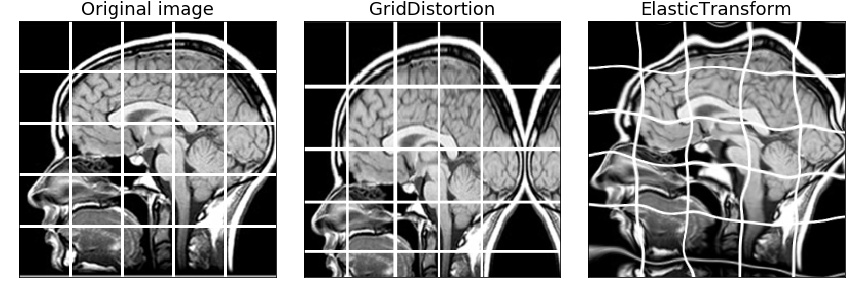
There are more interesting transformations, however. Take, for instance, grid distortion: we can slice the image up into patches and apply different distortions to different patches, taking care to preserve the continuity. Again, the labeling simply changes in the same way, and the result looks like this:

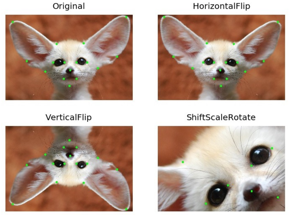
The same ideas can apply to other types of labeling. Take keypoints, for instance; they can be treated as a special case of segmentation and also changed together with the input image:

For some problems, it also helps to do transformations that take into account the labeling. In the image below, the main transformation is the so-called mask dropout: remove a part of the labeled objects from the image and from the labeling. But it also incorporates random rotation with resizing, blur, and a little bit of an elastic transform; as a result, it may be hard to even recognize that images on the right actually come from the images on the left:

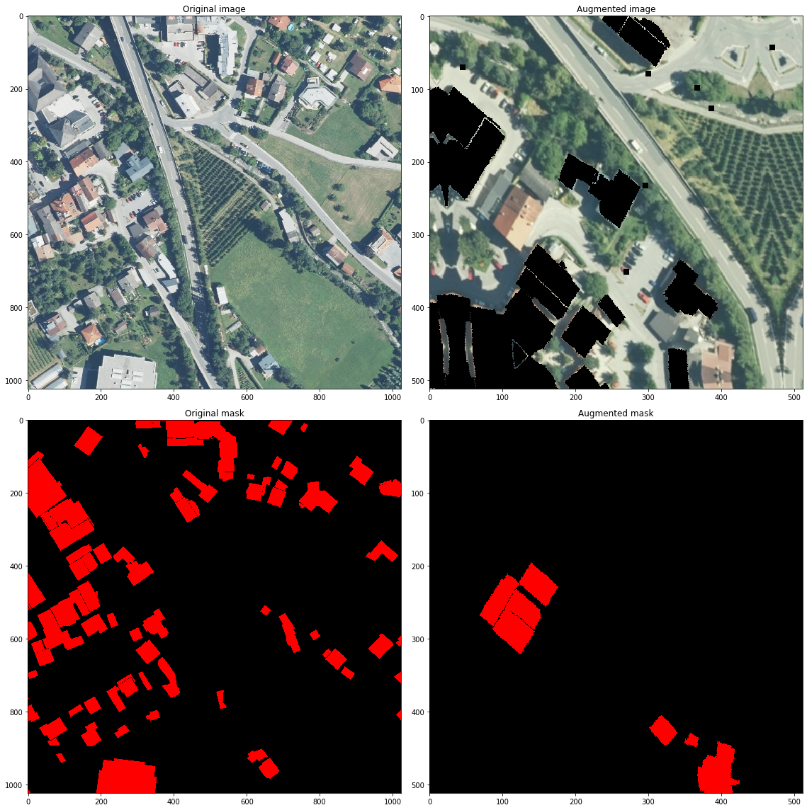
With such a wide set of augmentations, you can expand a dataset very significantly, covering a much wider variety of data and making the trained model much more robust. Note that it does not really hinder training in any way and does not introduce any complications in the development. With modern tools such as the Albumentations library, data augmentation is simply a matter of chaining together several transformations, and then the library will apply them with randomized parameters to every input image. For example, the images above were generated with the following chain of transformations:

light = A.Compose([
A.RandomSizedCrop((512-100, 512+100), 512, 512),
A.ShiftScaleRotate(),
A.RGBShift(),
A.Blur(),
A.GaussNoise(),
A.ElasticTransform(),
A.MaskDropout((10,15), p=1),
A.Cutout(p=1)
],p=1)

Not too hard to program, right?

Conclusion

Today, we have begun a new series of posts. I am starting a little bit further back than usual: in this post we have discussed data augmentations, a classical approach to using labeled datasets in computer vision.

Connecting back to the main topic of this blog, data augmentation is basically the simplest possible synthetic data generation. In augmentations, you start with a real world image dataset and create new images that incorporate knowledge from this dataset but at the same time add some new kind of variety to the inputs. Synthetic data works in much the same way, only the path from real-world information to synthetic training examples is usually much longer and more convoluted. So in a (rather tenuous) way, all modern computer vision models are training on synthetic data.

But this is only the beginning. There are more ways to generate new data from existing training sets that come much closer to synthetic data generation. So close, in fact, that it is hard to draw the boundary between “smart augmentations” and “true” synthetic data. Next time we will look through a few of them and see how smarter augmentations can improve your model performance even further.

Sergey Nikolenko
Head of AI, Synthesis AI