Today we have something very special for you: fresh results of our very own machine learning researchers! We discuss a case study that would be impossible without synthetic data: learning to recognize facial landmarks (keypoints on a human face) in unprecedented numbers and with unprecedented accuracy. We will begin by discussing why facial landmarks are important, show why synthetic data is inevitable here, and then proceed to our recent results.

Why Facial Landmarks?

Facial landmarks are certain key points on a human face that define the main facial features: nose, eyes, lips, jawline, and so on. Detecting such key points on in-the-wild photographs is a basic computer vision problem that could help considerably for a number of face-related applications. For example:

• head pose estimation, that is, finding out where a person is looking and where the head is turned right now;
• gaze estimation, a problem important for mobile and wearable devices that we discussed recently;
• recognizing emotions (that are reflected in moving landmarks) and other conditions; in particular, systems recognizing driver fatigue often rely on facial landmarks in preprocessing.

There are several different approaches to how to define facial landmarks; here is an illustration of no less than eight approaches from Sagonas et al. (2016) who introduced yet another standard:

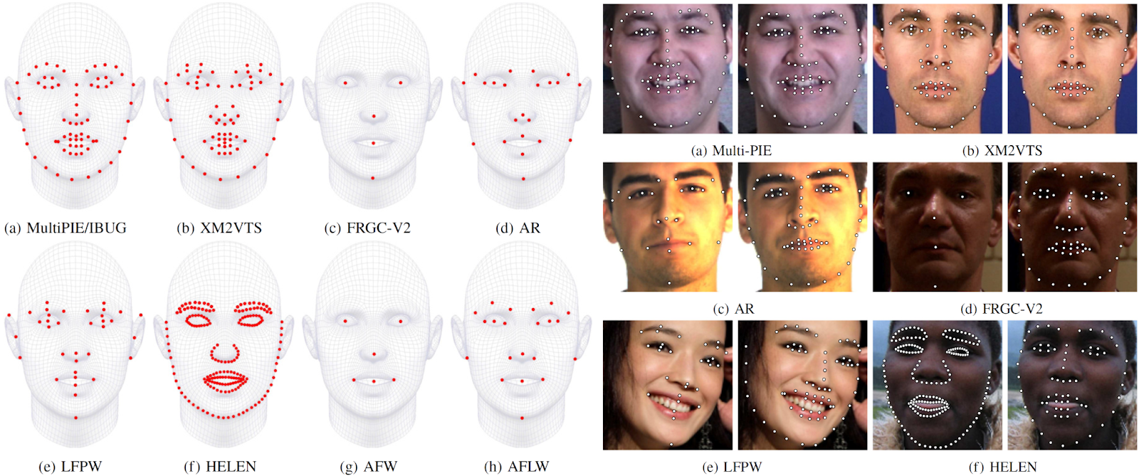
Their standard became one of the most widely used in industry. Named iBug68, it consists of 68 facial landmarks defined as follows (the left part shows the definitions, and the right part shows the variance of landmark points as captured by human annotators):

The iBug68 standard was introduced together with the “300 Faces in the Wild” dataset; true to its name, it contains 300 faces with landmarks labeled by agreement of several human annotators. The authors also released a semi-automated annotation tool that was supposed to help researchers label other datasets—and it does quite a good job.

All this happened back in 2013-2014, and numerous deep learning models have been developed for facial landmarks detection since then. So what’s the problem? Can we assume that facial landmarks are either solved or, at least, are not suffering from the problems that synthetic data would alleviate?

Synthetic Landmarks: Number does Matter

Not quite. As it often happens in machine learning, the problem is more quantitative than qualitative: existing datasets of landmarks can be insufficient for certain tasks. 68 landmarks are enough to get good head pose estimation, but definitely not enough to, say, obtain a full 3D reconstruction of a human head and face, a problem that we discussed very recently and deemed very important for 3D avatars, the Metaverse, and other related problems. 

For such problems, it would be very helpful to move from datasets of several dozen landmarks to datasets of at least several hundred landmarks that would outline the entire face oval and densely cover the most important lines on a human face. Here is a sample face with 68 iBug landmarks on the left and 243 landmarks on the right:

And we don’t have to stop there, we can move on to 460 points (left) or even 1001 points (right):

The more the merrier! If we are able to detect hundreds of keypoints on a face it would significantly improve the accuracy of 3D face reconstruction and many other computer vision problems.

However, by now you probably already realize the main problem of these extended landmark standards: there are no datasets, and there is little hope of ever getting them. It was hard enough to label 68 points by hand, the original dataset had only 300 photos; labeling several hundred points on a scale sufficient to train models to recognize them would be certainly prohibitive.

This sounds like a case for synthetic data, right? Indeed, the face shown above is not real, it is a synthetic data point produced by our very own Human API. When you have a synthetic 3D face in a 3D scene that you control, it is absolutely no problem to have as many landmarks as you wish. What’s even more important, you can easily play with the positions of these landmarks and choose which set of points gives you better results in downstream tasks—imagine how hard it would be if you had to get updated human annotations every time you changed landmark locations!

So at this point, we have a source of unlimited synthetic facial landmark datasets. It only remains to find out whether they can indeed help train better models.

Training on Synthetic Landmarks

We have several sets of synthetic landmarks, and we want to see how well we are able to predict them. As the backbone for our deep learning model we used HourglassNet, a venerable convolutional architecture that has been used for pose estimation and similar problems since it was introduced by Newell et al. (2016):

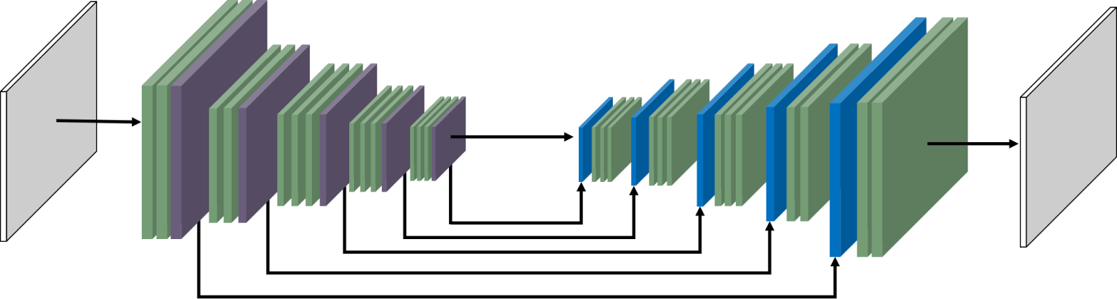
The input here is an image, and the output is a tensor that specifies all landmarks.

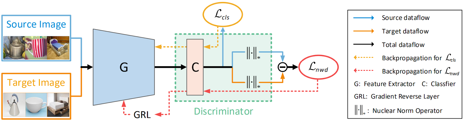
To train on synthetic data, we couple this backbone with the discriminator-free adversarial learning (DALN) approach introduced very recently by Chen et al. (2022); this is actually another paper from CVPR 2022 so you can consider this part a continuation of our CVPR ‘22 series.

Usually, unsupervised domain adaptation (UDA) works in an adversarial way by

• either training a discriminator to distinguish between features extracted from source domain inputs (synthetic data) and target domain inputs (real data), training the model to make this discriminator fail,
• or learning a source domain classifier and a target domain classifier at the same time, training them to perform the same on the source domain and as different as possible on the target domain while training the model to keep the classification results similar on the target domain.

DALN suggested a third option for adversarial UDA: it trains only one classifier, with no additional discriminators, and reuse the classifier as a discriminator. The resulting loss function is a combination of a regular classification loss on the source domain and a special adversarial loss on the target domain that is minimized by the model and maximized by the classifier’s weights:

We have found that this approach works very well, but we had an additional complication. Our synthetic datasets have more landmarks than iBug68. This means that we cannot use real data to help train the models in a regular “mix-and-match” fashion, simply adding it in some proportion together with the synthetic data. We could pose our problem as pure unsupervised domain adaptation, but that would mean we were throwing away perfectly good real labelings, which also does not sound like a good idea.  

To use the available real data, we introduced the idea of label transfer on top of DALN: our model outputs a tensor of landmarks as they appear in synthetic data, and then an additional small network is trained to convert this tensor into iBug68 landmarks. As a result, we get the best of both worlds: most of our training comes from synthetic data, but we can also fine-tune the model with real iBug68 datasets through this additional label transfer network.

Finally, another question arises: okay, we know how to train on real data via an auxiliary network, but how do we test the model? We don’t have any labeled real data with our newly designed extra dense landmarks, and labeling even a test set by hand is very problematic. There is no perfect answer here but we found two good ones: we test either only on the points that should exactly coincide with iBug landmarks (if they exist) or train a small auxiliary network to predict iBug landmarks, fix it, and test the rest. Both approaches show that the resulting model is able to predict dense landmarks, and both synthetic and real data are useful for the model even though the real part only has iBug landmarks.

Quantitative results

At this point, we understand the basic qualitative ideas that are behind our case study. It’s time to show the money, that is, the numbers!

First of all, we need to set the metric for evaluation. We are comparing sets of points that have a known 1-to-1 correspondence so the most straightforward way would be to calculate the average distance between corresponding points. Since we want to be able to measure quality on real datasets, we need to use iBug landmarks in the metric, not extended synthetic sets of landmarks. And, finally, different images will have faces shown at different scales, so it would be a bad idea to measure the distances directly in pixels or fractions of image size. This brings us to the evaluation metric computed as

where n is the number of landmarks, y_i are the ground truth landmark positions, f(x_i) are the landmark positions predicted by the model, and pupil are the positions of the left and right pupil of the face in question (this is the normalization coefficient). The coefficient 100 is introduced simply to make the numbers easier to read.

With this, we can finally show the evaluation tables! The full results will have to wait for an official research paper, but here are some of the best results we have now.

Both tables below show evaluations on the iBug dataset. It is split into four parts: the common training set (you only pay attention to this metric to ensure that you avoid overfitting), the common test set (main test benchmark), a specially crafted subset of challenging examples, and a private test set from the associated competition. We will show the synthetic test set, common test set from iBug, and their challenging test set as a proxy for generalizing to a different use case.

In the table below, we show all four iBug subsets; to get the predictions, in this table we predict all synthetic landmarks (490 keypoints in this case!) and then choose a subset of them that most closely corresponds to iBug landmarks and evaluate on it.

Model	Synthetic test set	Common test set	Challenging test set
Trained on synthetic data only	3.61	8.438	20.127
Trained on syn+real data with label adaptation	3.278	5.033	9.595
Unsupervised model with a discriminator	3.755	6.642	14.947
Supervised model trained on real data only		3.07	6.525

The table above shows only a select sample of our results, but it already compares quite a few variations of our basic model described above:

• the model trained on purely synthetic data; as you can see, this variation loses significantly to all other ways to train, so using real data definitely helps;
• the model trained on a mix of labeled real and synthetic data with the help of label adaptation as we have described above; we have investigated several different variations of label adaptation networks and finally settled on a small U-Net-like architecture;
• the model trained adversarially in an unsupervised way; “unsupervised” here means that the model never sees any labels on real data, it uses labeled synthetic data and unlabeled real data with an extra discriminator that ensures that the same features are extracted on both domains; again, we have considered several different ways to organize unsupervised domain adaptation and show only the best one here.

But wait, what’s that bottom line in the table and how come it shows by far the best results? This is the most straightforward approach: train the model on real data from the iBug dataset (common train) and don’t use synthetic data at all. While the model shows some signs of overfitting, it still outperforms every other model very significantly.

One possible way to sweep this model under the rug would be to say that this model doesn’t count because it is not able to show us any landmarks other than iBug’s, so it can’t provide the 490 or 1001 landmarks that other models do. But still — why does it win so convincingly? How can it be that adding extra (synthetic) data hurts performance in all scenarios and variations?

The main reason here is that iBug landmarks are not quite the same as the landmarks that we predict, so even the nearest corresponding points introduce some bias that shows in all rows of the table. Therefore, we have also introduced another evaluation setting: let’s predict synthetic landmarks and then use a separate small model (a multilayer perceptron) to convert the predicted landmarks into iBug landmarks, in a procedure very similar to label adaptation that we have used to train the models. We have trained this MLP on the same common train set.

The table below shows the new results.

Model	Synthetic test set	Common test set	Challenging test set
Trained on synthetic data only	3.61	4.777	13.115
Trained on syn+real data with label adaptation	3.278	3.825	7.53
Unsupervised model with a discriminator	3.755	5.008	11.834

As you can see, this test-time label adaptation has improved the results across the board, and very significantly! However, they still don’t quite match the supervised model, so some further research into better label adaptation is still in order. The relative order of the model has remained more or less the same, and the mixed syn+real model with label adaptation done with a small U-Net-like architecture wins again, quite convincingly although with a smaller margin than before.

Conclusion

We have obtained significant improvements in facial landmark detection, but most importantly, we have been able to train models to detect dense collections of hundreds of landmarks that have never been labeled before. And all this has been made possible with synthetic data: manual labeling would never allow us to have a large dataset with so many landmarks. This short post is just a summary: we hope to prepare a full-scale paper about this research soon.

Kudos to our ML team, especially Alex Davydow and Daniil Gulevskiy, for making this possible! And see you next time!

Sergey Nikolenko
Head of AI, Synthesis AI

P.S. Have you noticed the cover images today? They were produced by the recently released Stable Diffusion model, with prompts related to facial landmarks. Consider it a teaser for a new series of posts to come…