With the Christmas and New Year holidays behind us, let’s continue our series on how to improve the performance of machine learning models with synthetic data. Last time, I gave a brief introduction into domain adaptation, distinguishing between its two main variations: refinement, where synthetic images are themselves changed before they are fed into model training, and model-based domain adaptation, where the training process changes to adapt to training on different domains. Today, we begin with refinement for the same special case of eye gaze estimation that kickstarted synthetic data refinement a few years ago and still remains an important success story for this approach, but then continue and extend the story of refinement to other computer vision problems. Today’s post will be more in-depth than before, so buckle up and get ready for some GANs!

SimGAN in Detail

Let us begin with a quick reminder. As we discussed last time, Shrivastava et al. (2017) was one of the first approaches that successfully improved a real life model by refining synthetic images and feeding them to a relatively straightforward deep learning model. They took a large-scale synthetic dataset of human eyes created by Wood et al. (2016) and learned a transformation from synthetic images (“Source domain” in the illustration below) to real data (“Target domain” in the illustration below). To do that, they utilized a relatively straightforward SimGAN architecture; we saw it last time in a high-level description, but today, let’s dive a little deeper into the details.

Let me first draw a slightly more detailed picture for you:

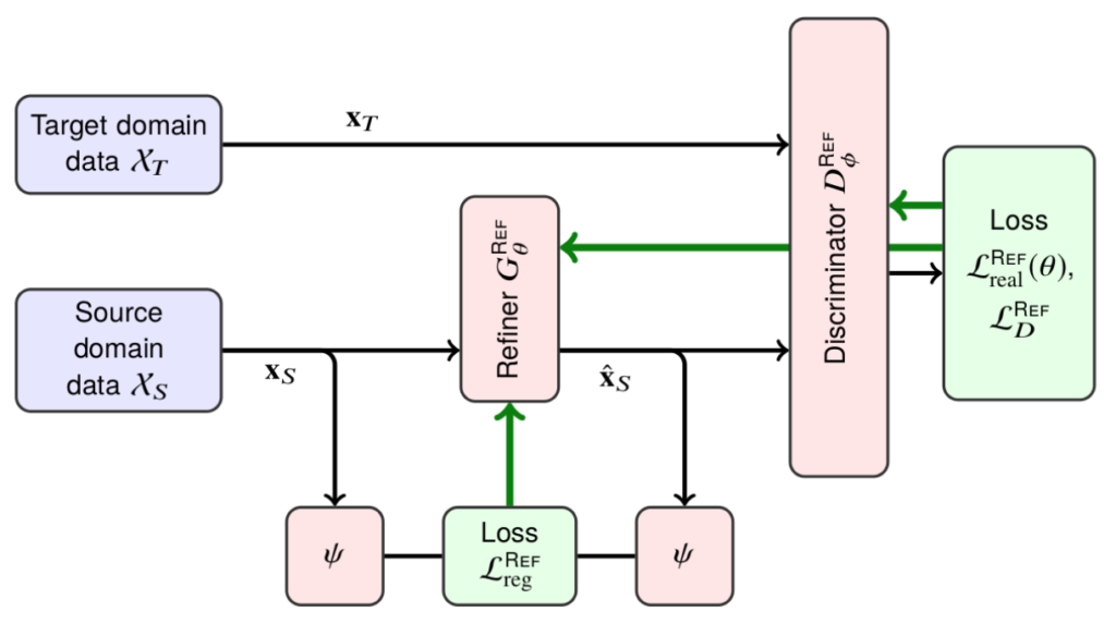
In the figure above, black arrows denote the data flow and green arrows show the gradient flow between SimGAN’s components. SimGAN consists of a generator (refiner) that translates source domain data into “fake” target domain data and a discriminator that tries to distinguish between “fake” and real target domain images.

The figure also introduces some notation: it shows that the overall loss function for the generator (refiner) in SimGAN consists of two components:

• the realism loss (green block on the right), usually called the adversarial loss in GANs, makes the generator fool the discriminator into thinking that the refined image is realistic; in a basic GAN such as SimGAN, this was simply the exact opposite of the binary cross-entropy loss for classification that the discriminator trains on;
• the regularization loss (green block on the bottom) makes the refinement process care for the actual target variable; it is supposed to make refinement preserve the eye gaze by preserving the result of some function ψ.

I will indulge myself with a little bit of formulas to make the above discussion more specific (trust me, you are very lucky that I can’t install a LaTeX plugin on this blog and have to insert formulas as pictures — otherwise this blog would be teeming with them). Here is the resulting loss function for SimGAN’s generator:

where ψ is a mapping into some kind of feature space. The feature space can contain the image itself, image derivatives, statistics of color channels, or features produced by a fixed extractor such as a pretrained CNN. But in case of SimGAN it was… in most cases, just an identity map. That is, the regularization loss simply told the generator to change as little as possible while still making the image realistic.

SimGAN significantly improved gaze estimation over state of the art. But it was a rather straightforward and simplistic GAN even for 2017. Since their inception, generative adversarial networks have evolved quite a bit, with several interesting ideas defining modern adversarial architectures. Fortunately, not only have they been applied to synthetic-to-real refinement, but we don’t even have to deviate from the gaze estimation example to see quite a few of them!

GazeGAN, Part I: Synthetic-to-Real Transfer with CycleGAN

Meet GazeGAN, an architecture also developed in 2017, a few months later, by Sela et al. (2017). It also does synthetic-to-real refinement for gaze estimation, just like SimGAN. But the architecture, once you lay it out in a figure, looks much more daunting:

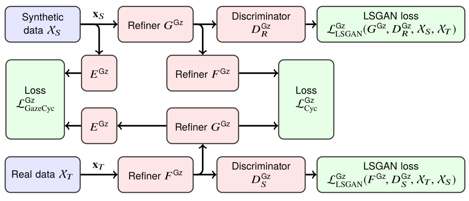
Let’s take it one step at a time.

First of all, the overall structure. As you can see, GazeGAN has two different refiners, F and G, and two discriminators, one for the source domain and one for the target domain. What’s going on here?

In this structure, GazeGAN implements the idea of CycleGAN introduced by Zhu et al. (2017). The problem CycleGAN was solving was unpaired style transfer. In general, synthetic-to-real refinement is a special case of style transfer: we need to translate images from one domain to another. In a more general context, similar problems could include artistic style transfer (draw a Monet landscape from a photo), drawing maps from satellite images, coloring an old photo, and many more.

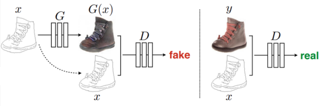
In GAN-based style transfer first introduced by the pix2pix model (Isola et al., 2016), you can have a very straightforward architecture where the generator does the transfer and the discriminator tries to tell apart fake pictures from real pictures. The main problem is how to capture the fact that the translated picture should be similar to the one generator received as input. Formally speaking, it is perfectly legal for the generator to just memorize a few Monet paintings and output them for every input unless we do something about it. SimGAN fixed this via a regularization loss that simply told the generator to “change as little as possible”, but this is not quite what’s needed and doesn’t usually work.

In the pix2pix model, style transfer is done with a conditional GAN. This means that both the generator and discriminator see the input picture from the source domain, and the discriminator checks both realism and the fact that the target domain image matches the source domain one. Here is an illustration (Isola et al., 2016):

This approach actually can be made to work very well; here is a sample result from a later version of this model called pix2pixhd (Wang et al., 2018), where the model is synthesizing a realistic photo from a segmentation map (not the other way around!):

But the pix2pix approach does not always apply. For training, this approach requires a paired dataset for style transfer, where images from the source and target domain match each other. It’s not a problem for segmentation maps, but, e.g., for artistic style transfer it would be impossible: Monet only painted some specific landscapes, and we can’t make a perfectly matching photo today.

Enter CycleGAN, a model that solves this problem with a very interesting idea. We need a paired dataset because we don’t know how to capture the idea that the translated image should inherit content from the original. What should be the loss function that says that this image shows the same landscape as a given Monet painting but in photographic form?..

But imagine that we also have an inverse transformation. Then we would be able to make a photo out of a Monet painting, and then make it back into a Monet — which means that now it has to match the original exactly, and we can use some kind of simple pixel-wise loss to make them match! This is precisely the cycle that CycleGAN refers to. Here is an illustration from (Zhu et al., 2017):

Now the cycle consistency loss that ensures that G(F(x))=x can be a simple L₂ or L₁ pixel-wise loss.

If you have a paired dataset, it would virtually always be better to use an architecture such as pix2pix that makes use of this data, but CycleGAN works quite well for unpaired cases. Here are some examples for the Monet-to-photo direction from the original CycleGAN:

In GazeGAN, the cycle is, as usual, implemented by two generators and two discriminators, one for the source domain and one for the target domain. But the cycle consistency loss consists of two parts:

• first, a simple pixel-wise L₁ loss, just like we discussed above:

• but second, we also need a special gaze cycle consistency loss to preserve the gaze direction (so that the target variable can be transferred with no change); for this, Sela et al. train a separate gaze estimation network E designed to overfit to the source domain as much as possible and predict the gaze very accurately on synthetic data; the loss makes sure E still works after going through a cycle:

GazeGAN, Part II: LSGAN, Label Smoothing, and More

Apart from the overall CycleGAN structure, the GazeGAN model also used quite a few novelties that had been absent in SimGAN but had already become instrumental in GAN-based architectures by the end of 2017. Let’s discuss at least a couple of those.

First, the adversarial loss function. As I mentioned above, SimGAN used the most basic adversarial loss: binary cross-entropy which is the natural loss function for classification. However, this loss function has quite a few undesirable properties that make it hard to train GANs with. Since the original GANs were introduced in 2014, a lot of different adversarial losses have been developed, but the two probably most prominent and most often used are Wasserstein GANs (Arjovsky et al., 2017) and LSGAN (Least Squares GAN; Mao et al., 2016).

I hope I will have a reason to discuss Wasserstein GANs in the future — it’s a very interesting idea that sheds a lot of light on the training of GANs and machine learning in general. But GazeGAN used the LSGAN loss function. As the title suggests, LSGAN uses the least squares loss function instead of binary cross-entropy. In the general case, it looks like

which means that the discriminator is trying to output some constant b on real images and some other constant a on fake images, while the generator is trying to convince the discriminator to output c on fake images (it has no control over the real ones). Naturally, usually one takes a=0 and b=c=1, although there is an interesting theoretical result about the case when b–c=1 and b–a=2, that is, when the generator is trying to make the discriminator maximally unsure about the fake images.

In general, trying to learn a classifier with the least squares loss is about as wrong as you can be in machine learning: this loss function becomes larger as the classifier becomes more sure in the correct answer! But for GANs, the saturation of the logistic sigmoid in binary cross-entropy is a much more serious problem. Even more than that, GazeGAN uses label smoothing on top of the LSGAN loss: while the discriminator aims to output 1 on real examples and 0 on refined synthetic images, the generator smoothes its target to 0.9, getting the loss function

this loss is applied in both CycleGAN directions, synthetic-to-real and real-to-synthetic. Label smoothing helps the generator to avoid overfitting to intermediate versions of the discriminator (recall that GANs are trained by alternating between training the generator and the discriminator, and there is no way to train them separately because they need each other for training data).

And that’s it! With these loss functions, GazeGAN is able to create highly realistic images of eyes from synthetic eyes rendered by a Unity-based 3D modeling engine. Here are some samples by Sela et al. (2017):

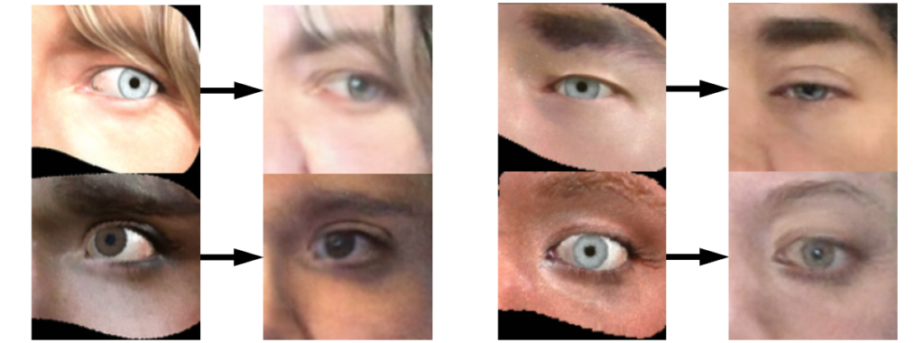
Note how this model works not only for the eye itself but also for the surrounding facial features, “filling in” even those parts of the synthetic image that were not there.

Conclusion

Today, we have discussed the gaze estimation problem in detail, taking this opportunity to talk about several important ideas in generative adversarial networks. Synthetic-to-real refinement has proven its worth with this example. But, as I already mentioned in the previous post, gaze estimation is also a relatively easy example: synthetic images of eyes that needed refining for Srivastava et al. were only 30×60 pixels in size!

GazeGAN takes the next step: it operates not on the 30×60 grayscale images but on 128×128 color images, and GazeGAN actually refines not only the eye itself but parts of the image (e.g., nose and hair) that were not part of the 3D model of the eye.

But these are still relatively small images and a relatively simple task, at least one with low variability in the data. Next time, we will see how well synthetic-to-real refinement works for other applications.

Sergey Nikolenko
Head of AI, Synthesis AI