Last time, I started a new series of posts, devoted to different ways of improving model performance with
synthetic data. In the first post of the series, we discussed probably the simplest and most widely used way to generate synthetic data: geometric and color data augmentation applied to real training data. Today, we take the idea of data augmentation much further. We will discuss several different ways to construct “smart augmentations” that make much more involved transformations of the input but still change the labeling only in predictable ways.

Automating Augmentations: Finding the Best Strategy
Last time, we discussed the various ways in which modern data augmentation libraries such as
Albumentations can transform an unsuspecting input image. Let me remind one example from last time:

Here, the resulting image and segmentation mask are the result of the following chain of transformations:
- take a random crop from a predefined range of sizes;
- shift, scale, and rotate the crop to match the original image dimension;
- apply a (randomized) color shift;
- add blur;
- add Gaussian noise;
- add a randomized elastic transformation for the image;
- perform mask dropout, removing a part of the segmentation masks and replacing them with black cutouts on the image.
That’s quite a few operations! But how do we know that this is the best way to approach data augmentation for this particular problem? Can we find the best way to augment, maybe via some automated meta-strategy that would take into account the specific problem setting?
As far as I know, this natural idea first bore fruit in the paper titled “
Learning to Compose Domain-Specific Transformations for Data Augmentation” by Stanford researchers Ratner et al. (2017). They viewed the problem as a sequence generation task, training a recurrent generator to produce sequences of transformation functions:

The next step was taken in the work called “
AutoAugment: Learning Augmentation Strategies from Data” by Cubuk et al. (2019). This is a work from Google Brain, from the group led by Quoc V. Le that has been working wonders with neural architecture search (NAS), a technique that automatically searches for the best architectures in a class that can be represented by computational graphs. With NAS, this group has already improved over the state of the art in basic convolutional architectures with
NASNet and the
EfficientNet family, in object detection architectures with the
EfficientDet family, and even in such a basic field as activation functions for individual neural units: the
Swish activation functions were found with NAS.
So what did they do with augmentation techniques? As usual, they frame this problem as a reinforcement learning task where the agent (controller) has to find a good augmentation strategy based on the rewards obtained by training a child network with this strategy:

The controller is trained by proximal policy optimization, a rather involved reinforcement learning algorithm that I’d rather not get into (
Schulman et al., 2017). The point is, they successfully learned augmentation strategies that significantly outperform other, “naive” strategies. They were even able to achieve improvements over state of the art in classical problems on classical datasets:

Here is a sample augmentation policy for ImageNet found by Cubuk et al.:

The natural question is, of course: why do we care? How can it help us when we are not Google Brain and cannot run this pipeline (it does take a
lot of computation)? Cubuk et al. note that the resulting augmentation strategies can indeed transfer across a wide variety of datasets and network architectures; on the other hand, this transferability is far from perfect, so I have not seen the results of AutoAugment pop up in other works as often as the authors would probably like.
Still, these works prove the basic point: augmentations can be composed together for better effect. The natural next step would be to have some even “smarter” functions. And that is exactly what we will see next.
Smart Augmentation: Blending Input Images
In the previous section, we discussed how to chain together standard transformations of input images in the best possible ways. But what if we take one step further and allow augmentations to produce more complex combinations of input data points?
In 2017, this idea was put forward in the work titled “
Smart Augmentation: Learning an Optimal Data Augmentation Strategy” by Irish researchers Lemley et al. Their basic idea is to have two networks, “Network A” that implements an augmentation strategy and “Network B” that actually trains on the resulting augmented data and solves the end task:

The difference here is that Network A does not simply choose from a predefined set of strategies but operates as a generative network that can, for instance, blend two different training set examples into one in a smart way:

In particular, Lemley et al. tested their approach on datasets of human faces (a topic quite close to our hearts here at Synthesis AI, but I guess I will talk about it in more details later). So their Network A was able to, e.g., compose two different images of the same person into a blended combination (on the left):

Note that this is not simply a blend of two images but a more involved combination that makes good use of facial features. Here is an even better example:

This kind of “smart augmentation” borders on synthetic data generation: the resulting images are nothing like the originals. But before we turn to actual synthetic data (in subsequent posts), there are other interesting ideas one could apply even at the level of augmentation.
Mixup: Blending the Labels
In smart augmentations, the input data is produced as a combination of several images with the same label: two different images of the same person can be “interpolated” in a way that respects the facial features and expands the data distribution.
Mixup, a technique introduced by MIT and FAIR researchers
Zhang et al. (2018), looks at the problem from the opposite side: what if we mix the labels together with the training samples? This is implemented in a very straightforward way: for two labeled input data points, Zhang et al. construct a convex combination of both the inputs and the labels:

The blended label does not change either the network architecture or the training process: binary cross-entropy trivially generalizes to target discrete distributions instead of target one-hot vectors. To borrow an illustration from Ferenc Huszar’s
blog post, here is what mixup does to a single data point, constructing convex combinations with other points in the dataset:

And here is what happens when we label a lot of points uniformly in the data:

As you can see, the resulting labeled data covers a much more robust and continuous distribution, and this helps the generalization power. Zhang et al. report especially significant improvements in training GANs:

By now, the idea of mixup has become an important part of the deep learning toolbox: you can often see it as an augmentation strategy, especially in the training of modern GAN architectures.
Self-Adversarial Training
To get to the last idea of today’s post, I will use YOLOv4, a recently presented object detection architecture (
Bochkovskiy et al., 2020). YOLOv4 is a direct successor to the famous YOLO family of object detectors, improving significantly over the previous YOLOv3. We are, by the way, witnessing an interesting controversy in object detection because YOLOv5 followed less than two months later, from a completely different group of researchers, and without a paper to explain the new ideas (but with the code so it is not a question of reproducing the results)…
Very interesting stuff, but discussing it would take us very far from the topic at hand, so let’s get back to YOLOv4. It boasts impressive performance, with the same detection quality as the above-mentioned EfficientDet at half the cost:

In the YOLO family, new releases usually obtain a much better object detection quality by combining a lot of small improvements, bringing together everything that researchers in the field have found to work well since the previous YOLO version. YOLOv4 is no exception, and it outlines several different ways to add new tricks to the pipeline.
What we are interested in now is their “Bag of Freebies”, the set of tricks that do not change the performance of the object detection framework during inference, adding complexity only at the training stage. It is very characteristic that most items in this bag turn out to be various kinds of data augmentation. In particular, Bochkovskiy et al. introduce a new “mosaic” geometric augmentation that works well for object detection:

But the most interesting part comes next. YOLOv4 is trained with self-adversarial training (SAT), an augmentation technique that actually incorporates adversarial examples into the training process. Remember this famous picture?

It turns out that for most existing artificial neural architectures, one can modify input images with small amounts of noise in such a way that the result looks to us humans completely indistinguishable from the originals but the network is very confident that it is something completely different; see, e.g.,
this OpenAI blog post for more information.
In the simplest case, such adversarial examples are produced by the following procedure:
- you have a network and an input x that you want to make adversarial; suppose you want to turn a panda into a gibbon;
- formally, it means that you want to increase the “gibbon” component of the network’s output vector (at the expense of the “panda” component);
- so you fix the weights of the network and start regular gradient ascent, but with respect to x rather than the weights! This is the key idea for finding adversarial examples; it does not explain why they exist (it’s not an easy question) but if they do, it’s really not so hard to find them.
So how do you turn this idea into an augmentation technique? Given an input instance, you make it into an adversarial example by following this procedure for the current network that you are training. Then you train the network on this example. This may make the network more resistant to adversarial examples, but the important outcome is that it generally makes the network more stable and robust: now we are explicitly asking the network to work robustly in a small neighborhood of every input image. Note that the basic idea can again be described as “make the input data distribution cover more ground”, but by now we have come quite a long way since horizontal reflections and random crops…
Note that unlike basic geometric augmentations, this may turn out to be a quite costly procedure. But the cost is entirely borne during training: yes, you might have to train the final model for two weeks instead of one, but the resulting model will, of course, work with exactly the same performance: the model architecture does not change, only the training process does.
Bochkovskiy et al. report this technique as one of the main new ideas and main sources of improvement in YOLOv4. They also use the other augmentation ideas that we discussed, of course:

YOLOv4 is an important example for us: it represents a significant improvement in the state of the art in object detection in 2020… and much of the improvement comes directly from better and more complex augmentation techniques! This makes us even more optimistic about taking data augmentation further, to the realm of synthetic data.
Conclusion
In the second post in this new series, we have seen how more involved augmentations take the basic idea of covering a wider variety of input data much further than simple geometric or color transformations ever could. With these new techniques, data augmentation almost blends together with synthetic data as we usually understand it (see, e.g., my previous posts on this blog:
one,
two,
three,
four,
five).
Smart augmentations such as presented in Lemley et al. border on straight up automated synthetic data generation. It is already hard to draw a clear separating line between them and, say, synthetic data generation with GANs as presented by
Shrivastava et al. (2017) for gaze estimation. The latter, however, is a classical example of domain adaptation by synthetic data refinement. Next time, we will begin to speak about this model and similar techniques for domain adaptation intended to make synthetic data work even better. Until then!
Sergey Nikolenko
Head of AI, Synthesis AI